All connections available in the Steel Connection module can be designed using all combinations or envelopes created from those combinations.
The possibility to choose how to use the combinations in the design process is available in the Design Assumptions dialog.
By selectingEnvelopes method, the calculation will be performed using only the combinations that provide Max/Min of the design forces using certain filtering criteria done in Advance Design Steel connection.
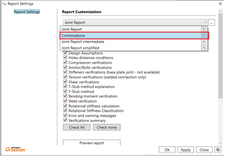
The envelopes that are considered now in calculation can be seen inside the new Combinations report or inside detailed or intermediate reports in the Load combinations chapter.
The Combinations report added to the available report list for each joint type will display only theLoad combinations description chapter, which will provide an easier and faster way to access the envelope list.
As have been mentioned, there are two options possible: All and Envelopes.
Now let’s see how the selection affects the behavior during calculation process.
Combinations = All
For Combinations set on “All”, the Advance Design Steel Connection is using all the combinations generated to design the connection.
Example:
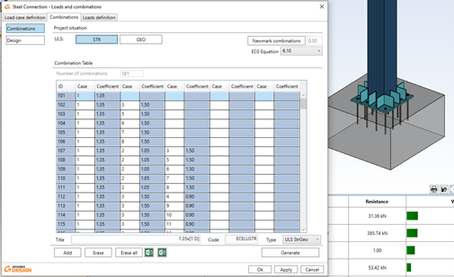
For the Base Plate connection for a tubular column as on the picture below, the number of combinations is 181, and all are used for design calculations. It influences the report (as a table listing all the combinations is long), but the most important is that due to the number of combinations, the calculation time is relatively long.
Combinations = Envelopes
For Combinations set as “Envelopes” the module will calculate the connection using just some of the combinations which are fulfilling certain criteria.
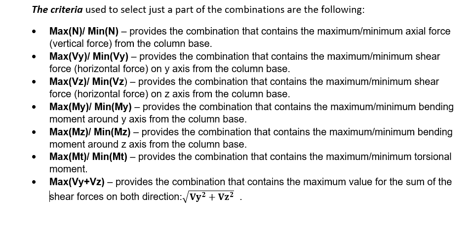
The criteria used to select just a part of the combinations are the following:
Based on these criteria, Advance Design Steel Connection module is selecting the combinations that compliant with one or more criteria and does the design calculations based on the selected combinations.
The calculation time decreases, and the report is much more compact as only the selected combinations will be listed.
Example:
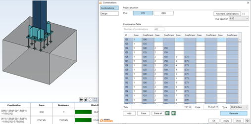
For the Base Plate connection for a tubular column as on the picture below (having more load cases that the previous example), the number of combinations is 482. But this time calculations are done with “Envelopes” of combinations.
Even there are 482 combinations, thanks to the envelopes, the calculation time is less than for the previous example. And in addition, the report does not have pages full of combination tables and it is generated much faster. The Load combinations description table on the report contains now only several combinations that are fulfilling one or more criteria. And the connection is verified using these combinations
As the 2022 version of GRAITEC Advance Design introduced the Crane Moving Loads feature, in this short article we will take a look at the moving loads available in Advance Design – the Traffic load and the new Crane load. As the traffic load generator has been available for a long time, I will present only brief information about it and focus mainly on crane loads.
Moving load panel on the ribbon
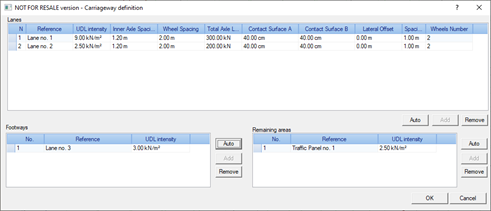
Let us start with the traffic load. The traffic load generator enables us to create traffic loads on road bridges according to EN1991-2 (Section 4). In order to create the appropriate traffic loads on the road bridge (on planar elements), we define graphically the elements composing the carriageway: one or several traffic lanes, remaining areas and footways or cycle-tracks.
Carriageway definition
The next step is to add a Traffic loads family and select the appropriate load model, according to the provisions of the Eurocode. Five load groups are available, containing respectively:
gr1a – combination of the concentrated loads (Tandem Systems) and the Uniformly Distributed Load (UDL System) with the uniformly distributed load on footways.
gr1b – a couple of concentrated loads that represent a single axle of a truck, for creating concentrated forces along the lane.
gr2 – combination of the concentrated loads (Tandem Systems) and the Uniformly Distributed Load (UDL System) with braking and acceleration forces and centrifugal forces.
gr3 – uniformly distributed load on footways.
gr4 – uniformly distributed load on footways and traffic panels.
Traffic load model selection
After automatically assigning the load parameters to the roadway, we are ready for load generation in the model.
Carriageway load parameters
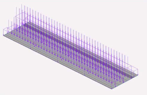
Depending on the load model selected, this results in load cases that include uniform loads as well as a series of consecutive steps in the position of the concentrated forces from the vehicle wheels.
Uniform loads and moving loads from vehicle (all steps are shown)
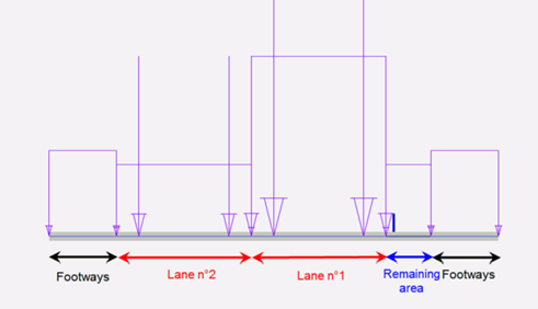
Loads in section for one of the selected steps
For loads from cranes, the process is somewhat similar. The first stage consists in defining graphically the route of the crane forces – it can be a single polyline to model the forces moving along a single rail (for monorail crane modelling) or two parallel lines to model the route for the forces from two trucks on both sides of the bridge crane.
Runway for the bridge crane placed on two beams
The next step is to add a Crane object. It is used to describe the geometry, such as the number and spacing of the wheels, and to describe the forces from the wheels.
Basic crane geometrical data
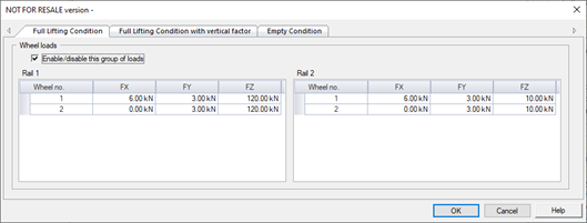
In the simplest case, the forces on each wheel can be defined manually, separately for each wheel. But it is also possible to use three different automatic methods, so that the wheel forces are automatically determined according to the rules of the standard.
Choice of force generation method
We have three methods available for the automatic determination of forces:
By crane loads(EN 1991-3) – for defining wheel loads automatically on the basis of entered crane loads, by using Eurocode EN 1991-3 rules. In this method several loads of different origin (e.g. loads from crane self-weight, from the weight of the load, from braking forces, etc.) are separately entered for each wheel. These load components are combined with the dynamic factors and the final wheel forces are determined. As the result this method gives several groups of load sets (ULS Group 1 to 6), according to the EN 1991-3.
By crane parameters (EN 1991-3) – for defining wheel load automatically on the basis of entered crane parameters, by using the Eurocode EN 1991-3 rules. The main difference compared to the previous method is that the values for each wheel are not entered, but the crane parameters (like self-weight of the bridge, self-weight of the trolley and the crane capacity) are given. The output is the same as for the previous method – six groups with sets of forces for each wheel.
By crane parameters (ASCE/NBCC) – similar to the previous one, so we do not enter the forces on individual wheels, but such loads are calculated automatically on the basis of entered crane parameters. But this time the method of automatic load generation is based on the general method, related to US/CAN standards (especially ASCE). But it is worth to mention, that the load generation rules are generic and are essentially independent of any standard.
Groups of loads per wheel calculated acc. By crane parameters (ASCE/NBCC) method
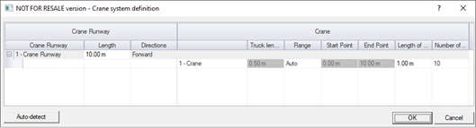
With the crane runway and the crane with the forces on the wheel, we can proceed to the next step, which is the definition of the load family. Here we determine the range of crane movement and the number/length of moving load steps.
Definition of move parameters for crane load family
The generation of crane moving cases is done automatically after using a ‘Generate’ command available when right click on the Crane Load case family. After it is run a set of moving load cases are generated, separately for each crane and each step position. They contain the forces from all wheels in a given position. Depending on the definition of the crane, these are both vertical forces and horizontal transverse or longitudinal (from braking) forces.
Load cases for each wheel position with forces
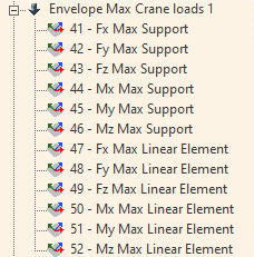
Together with the load case generation, sets of force envelopes from all force positions are also generated.
Automatically created envelopes
Importantly, we can define more than one crane and place them on the same or different runways. In this case, the program will generate for each crane a series of all force positions and then, when the envelope is generated, only the possible combinations of crane positions are considered.
One of the combinations of positions of 2 bridge cranes on the same runway
The final load combinations are defied by using typical load cases (dead, live, wind…) and Crane Envelopes. This is particularly important when there are a large number of crane steps and especially many cranes, as the final combinations consider only a dozen or so envelopes instead of thousands of crane position combinations.
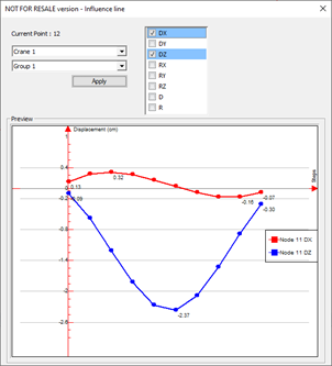
The static calculation and the results for the combination cases do not differ from other load types and you can check the results for each crane position as well as for the envelope of the crane forces. Specific to crane is a new type of graphical output – the influence line diagram. It shows graphically the value of the result at a given point for all successive positions of the crane. Although in this version of the program the influence line diagram can only be displayed for displacements in structure nodes, it is one of the additional tools useful when analyzing the results.
June 1st we released our products for their 2022 versions, this covers the entire Graitec portfolio, well within that there are few things that stand out to me coming from the Steel detailing and design background, that sound a clear intention of Graitec in this area.
The first one is within our analysis engine ‘Advance Design’, the New feature of Cold Formed Design to EC3. This is a Game changer for those engineers using portal frame constructions and trying to design the most efficient systems for those structures.
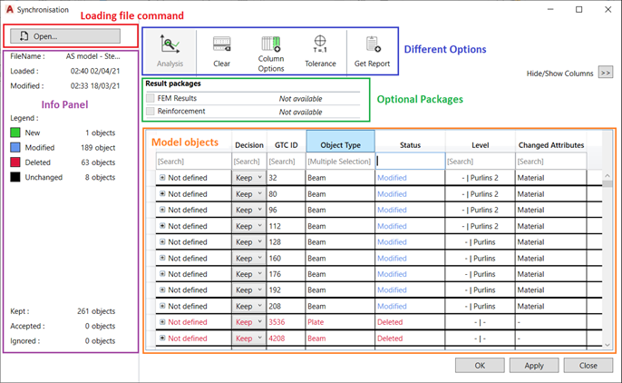
The next one is more in the link between our Advance Design platform and Autodesk Advance Steel for the transfer of model data, for this version we have a Newly design GUI and Mechanism for the Synchronization of Data using the Graitec GTCX file format. This new interface allows form many options to optimise what you wish to transfer and sync,
Figure 1-Example of new Dialog
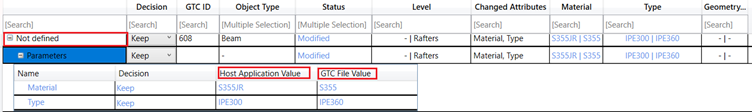
Within the file and the options available we have the ability to have a dedicated object ID, object type, Status display for New/Modified/Deleted, Material, Geometry, Element Type.
Figure 2-example of column types
Having all these options, we now have also filter options available, to help you dig down and only see the data you require.
Figure 3- filter example.
Also, the file has now the option to contain the level of the element within the model space. It has two options to show the host location and the allocated level in the GTCX itself.
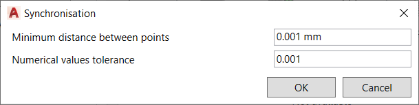
Also, all important one for model Tolerance, this allows for the user to control during the Sync process the variation between the model elements is acceptable, based upon those numeric values.
Figure 4- tolerance example
Concrete elements are now also considered for the GTCX file and the transfer, presently standard column, and beam shapes for this version, but sure other more complex shape definitions will be added to this new feature.
There are a lot more elements and options to the GTCX and the New Sync process, these are explained in depth in the what’s new, that is available to customers via the Graitec Advantage site.
Powerpack Premium Steel – Stairs and Railings
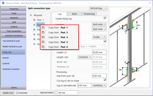
Within the premium model, particularly for Stairs and Railings we have a great new feature for those working with panelised balustrades/railings, that is the inclusion of ‘Lugs’ to the panels.
We can now add vertical and horizonal/incline lugs.
This may only look like a small feature but for those of us that have to detail these, this will be a real time saver.
Figure 5-Lugs dialog – perpendicular/incline to rail
Figure 6- Lugs – vertical to post.
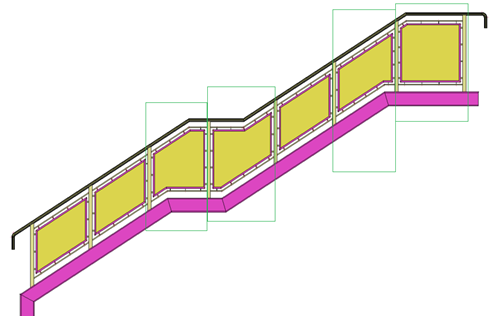
Anther part of the railings in the actual placement of panels within the rail, previously there where some limits on what we could achieve, but again the development team have worked on this to improve this function to accommodate more complex arrangements.
Figure 7- complex panel shaping
This also works with the frames type panels as well.
Figure 8- framed types
A new option is to allow for the user to turn off the top rail and still have the panels, this can be useful in the situation of external fencing panels and picket type fencing arrangements.
Figure 9- fencing arrangement/ Stairs/ pickets etc.
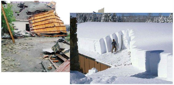
Climatic loads are a specific type of imposed loads to which almost every building object is exposed. Their nature and value is closely related to the type, geometry and location of the object. When preparing the design, the designer is obliged to include these loads in his calculations.
It has already happened in the past that incorrect consideration of this influence has led to disasters or failures. This aspect is often simplified or omitted due to a certain laboriousness of the determination of loads (especially wind loads) and their transfer to the calculation model, which will be the main subject of this article.
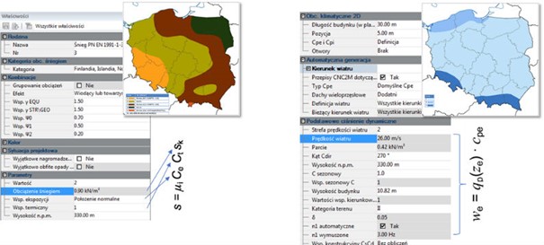
The current basis for the determination of climatic loads are Eurocode standards EN 1991-1-3 for snow loads and EN 1991-1-4 for wind loads.
In a similar way, these standards first determine the effect of the building location on the size of the characteristic load and divide the country into snow and wind load zones, respectively. The next step is to determine the nature of the load resulting from the geometry of the building itself – for wind it will be the external pressure zones and their distribution, while for snow it will be the roof shape factor. The whole is thus a basis and a relatively clear instruction for the determination of the ultimate snow and wind loads.
Automatic generation of loads in an FEA model
If the designer would like to determine these loads manually and apply them to the object in the calculation program, he has to reckon with a very labour-consuming task, mainly due to a multitude of coefficients leading to the final value and it is, so to say, complicated for even the simplest object. For example – we have to consider several wind directions, determine the range of external pressure zones, take into account the internal pressure, the value of pressure in individual zones, and to top it all off we have to take into account a number of dozens of variables and values (from dimensions, to location, to factors related to exposure, direction, terrain, etc.). The worst thing is that the whole thing is then drastically sensitive to change – a small change in the geometry of the building leads to a change in the external pressure zones.
Unfortunately, in most calculation programs we are forced to determine these actions manually and apply them in the form of loads to the FEM model of the structure, which often also requires us to prepare the model itself. Advance Design software has an automatic climatic load generator based on Eurocode, working on the principle of geometry discretisation to the appropriate standard schemes. The user does not have to impose any parameters connected with building geometry.
Above is a general diagram of how a climate load generator works (using wind as an example). Step 1 is practically just the preparation of the FE model for any subsequent analysis. However, it is important that the whole object is clad with cladding, i.e. panels, which do not have any mechanical properties but are only supposed to distribute the surface load on the structural elements. Their geometry is presented in step 2 – on this basis the program recognises the shape of the object and applies appropriate load schemes. Step 3 is the determination of the external pressure zones and the load values which are distributed from the cladding to the members and shells in step 4. In step 5 the final result, the wind load on the structure, is presented.
All these operations take place automatically and one could say that they are by default invisible for the user – the designer only prepares the geometry and as a result he gets the structure loaded by climatic actions. Importantly, any change to the design (geometry, assumptions etc.) allows the loads to be automatically updated to the current state of the model.
Guide to Advance Design generator
The 2020 version of the programme introduced a number of tools allowing to easily generate all cladding in an extremely short time e.g. by selecting linear/surface elements, by drawing or copying.
The cladding determines in which direction (x/y/xy/other defined by angle) it will distribute the load applied to its surface. It also determines certain parameters related to climatic loads.
The loads are determined from the parameters specified in the load cases.
The operation itself is trivial – the parameters we need to establish are those that are not possible to establish from the model but result from the project assumptions (altitude, thermal coefficient, terrain category, etc.).
After these two operations (cladding and load cases), the program is ready to generate loads. It will create exactly as many load cases as necessary from the point of view of uniform/nonuniform snow or different pressure values in the individual zones.
CNC2M – additional provisions for wind loads
Very importantly, the program implements the provisions of the CNC2M document. This document is a kind of annex to the French standars but it is universal in its nature regardless of the country. It defines rules for determining zones and pressure values for buildings much more complicated than those included in the general provisions of Eurocode, e.g. L-shaped or C-shaped buildings, awning canopies, additional provisions for wind shelters. In Poland we are not obliged to use such provisions, but it is a much more reliable approach than using a simple cuboid “cube” model for the whole building.
If you are new to Graitec Advance Design community then in this article we will draw your attention to useful tools that you may not have noticed in your first few weeks of work, but which can help you to complete your projects faster and more conveniently.
Generate, not draw …
One of Advance Design’s favorite features for advanced users is the ” … on selected” from the context menu under the right mouse button (PPM). These capabilities are available by selecting one or more elements. In this way you can quickly apply loads, insert supports, generate points, connections …. It couldn’t be easier.
2. Stay up to date with the parameters of the FEA model…
Another solution that is ideal to use when working with a model is the “Hint Label”. Its advantage is that it can be turned on and off via the “status bar” (see screenshot below) but it is also configurable. This way you can e.g. check the length of an element, coordinates of end points or corners of an object. Why is this so important? With “tooltips” there is less clicking (e.g. the “measure length” function) or “reading” into the parameters in the properties window…
3 Hide/Display FEA model objects with one click…
Finally, I chose a function that I as a user myself discovered very late…. i.e. access to the shortcut in the context menu (PPM) “Display…”. This is essentially a shortcut to the object display settings. What I liked about it is that I can “peel” the model of loads, cladding etc without having to click on the “Project Browser” which takes my attention away from the model content. In conjunction with the “isolate” function I can get at objects that are not system related.
Among the many functions constantly used when working with FEM models are such basic ones as object selection and filtering, i.e. controlling whether objects are visible or hidden. And while every FEM analysis program has these functions, what makes Advance Design stand out is its ease of use. So, let’s take a look at a few possibilities and see how easy we can use them.
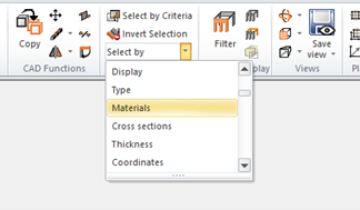
Leaving aside the graphical selection, let us first look at the simplest selection, that is, by basic criteria.
Criteria selection is the most basic type of selection – for example, when you want to select all elements of a particular cross-section or material or thickness in a modeled structure. In this case, simply select the relevant criterion, for example material, from the list. A window opens automatically in which you can enter a criterion – for example, select one or more materials from a list.
Among the many such critters available it is worth noting two: by System and by Name, as are extremely useful for a quick selection, especially if we have defined systems and subsystems and modified the default element names.
Other interesting quick selection criteria are Previous selection, which is the restoration of a previously existing selection, and Vicinity, which selects objects that are in contact with the currently selected items.
But what if we want to combine multiple criteria? Then we simply open the Select by Criteria window (for example by using ALT+S shortcut) and on each tab choose the criteria we want to use. For example, when you want to select IPE 300 and IPE360 profiles that simultaneously belong to a system called Front Structure. Just select these options from the list and press OK.
Interestingly, with a single click, you can change the default setting that selects items that meet all criteria (Intersection mode) to a setting that selects items that meet at least one of the selected criteria (Union mode). In addition, the operation can be performed on an existing selection. As you can see complex criteria are very easy to operate. As mentioned earlier, splitting the model into systems makes the work much easier. For example, when we want to select elements from a given system, we just need to do it from the Project browser level.
Using the same method, you can instantly hide or isolate a section of the model. Furthermore, you can hide/show objects (including those contained in systems) even faster simply by double-clicking on the Project browser in the list. On this picture just by few quick double clicks on the Project browser only columns and rafters are displayed.
All of these are simple operations, but they make working in Advance Design seamless because of their easy access and simple use.
Often the objects which we design require a more detailed analysis at the level of a specified fragment of the structure or element. For this purpose, often the whole object is modelled for the purpose of vertical element dimensioning, and horizontal elements such as floors are designed in a separate model, assuming their certain static scheme as faithfully as possible reflecting the global behaviour of these separated elements.
The problem begins to appear when the separated element must be loaded also with the remaining fragment of the structure, which we wanted to get rid of in order to reduce the large model. For the simplest example – I would like to analyse a complicated foundation slab – its separation from the model will not help me much, because loads which dimension it are transferred from the whole structure by means of columns or walls. The simple conclusion from this…I can isolate the slab as long as I load it according to the building scheme.
Advance Design allows you to exchange the support reactions of one model for loads generated in another model.
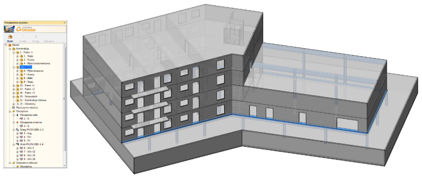
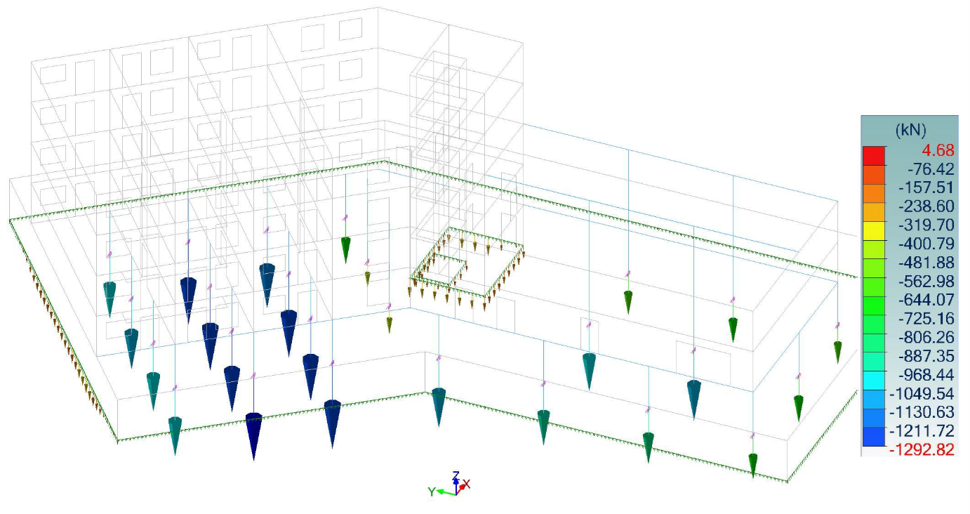
Fig. 1. Model of a simple residential and commercial building in Advance Design
At the moment I have a model of the entire building, which I can easily solve. However, I would like to divide the model e.g. into an underground and an aboveground part or into a foundation slab and the remaining part of the building. Maybe I need to analyse the foundation slab in detail and I need to reduce the size of the model to gain calculation time. Maybe I would like to divide the work into 2 workstations and leave the development of the ground slab to one of the co-workers and deal with the vertical elements of floor -1 or higher I am able to do this by creating, in a way, 2 independent models (e.g. of the said underground and aboveground part). The problem arises in the fact that the aboveground part will load the underground part, and I have just removed it from the model.
Fig. 2. Two independent FEA models
2 Foundation slab modelled on an elastic foundation, the part above the foundation slab supported by nominal rigid supports. At this point I can solve model one – i.e. the part above the foundation slab – without a problem.
Fig. 3. Reactions (vertical) from permanent loads
Saving reactions to a file and importing them in another task
Above are examples of support reactions from permanent loads. Of course, we can transfer all reactions (displacement/rotation) from all cases.
Please note that reactions are usually presented as an inverse vector, i.e. as a response of a support – here, however, our vertical reaction is directed downwards, as it is later to be a load on a foundation slab. The reverse of reactions can be reversed by changing the program settings in the results tab by switching off the option “Include reactions on supports”. On the BIM tab, the user can export the reactions to a text file and import them into the foundation slab model in the same way. The load cases and the position of forces in space are preserved.
Fig. 4. Reactions imported into the foundation slab model
Importantly, I can import reactions at any time, meaning potential changes to the output model are not threatening. I can also modify the geometry of the foundation slab freely – the loads are not associated with it, they are in a specific space in the model and load the element underneath them. The forces are in the same load cases as in the original model so the combinations do not change. I could, however, combine the loads differently because in a smaller, detailed foundation slab design I will be able to successfully prepare more combinations.
The only thing I would like to point out is that it is necessary to separate structural elements sensibly. Their work under loads may be influenced by the elements that we have removed. That is, in addition to transferring loads, they also stiffen the component under consideration and change its working character somewhat. It is relatively correct to separate the whole storey.
This method can also lead to a kind of phasing of the structure.
Graitec, as a global software editor in the Design, Structural, Fabrication, and Data Management arena organizes an international contest dedicated to structural engineers and design offices.
The award is for the best practical use of Advance Design in Steel / Timber / Concrete design projects. This contest is open to customers and students who want to showcase their experience and technical knowledge through a project executed in Advance Design software. The projects will be judged by a professional jury. The final nominees and the winning projects will be made public to a wide audience through extensive marketing including social media.
• 30.7.2021 Entries close – Deadline for project submission
• 10.9.2021 Project Confirmation – Confirmation and announcement of projects accepted
• 11.10.2021 Jury Deliberation – Selection of winners
• 19.10.2021 Announcement of Results – Announcement of winners at the Advance Design User Summit 2021
Contest criteria:
The independent contest jury will gather in October 2021 to evaluate the projects. The judging will be done under the guidance of a dedicated Graitec Group representative. The representative is in charge of the contest. The jury will evaluate the projects taking the following criteria into consideration:
Technical level of the design, detailing and/or calculations.
Originality and prestige of the project.
Attractiveness, detail and presentation of the project.
Optimal use of software’s functionality.
The “story” behind the project – difficulties overcome, innovative approaches, benefits gained, etc.
Jury:
An independent and international jury composed of academics and professionals in the field will judge the submitted entries. Meet the members of our jury:
Francis Guillemard – Jury Chairman / GRAITEC President of the Group and Chairman of the board / France
Rawad Assaf / ISSAE – CNAM Liban/ Lebanon
Olivier Chappat / Bouygues Bâtiment Ile-de-France / France
Piotr Nazarko / Rzeszow University of Technology / Poland
Rodrigue Coyere / EIFFAGE CONSTRUCTION Structural design office / France
Daniel Bitca / Technical University of Civil Engineering Bucharest / Romania
Jiri Bendl, GRAITEC, Vice President SIMULATE comments: “Through the Advance Design Award organizations we want to reward our customers for being members of the ever-growing SIMULATE community and we want to encourage students to use the best possible tools for structural analysis. It is a great pleasure for me to be part of this project!”
About GRAITEC
Founded in 1986, GRAITEC is an international group (13 countries worldwide – 48 offices) helping construction and manufacturing professionals to successfully achieve their digital transformation by providing BIM and Industry 4.0 software and consultancy. GRAITEC is a developer of high-performance BIM applications as well as an Autodesk Platinum Partner in Europe and Gold Autodesk Partner in North America and Russia. With more than 550 employees including 200 BIM consultants, GRAITEC is an innovation-focused company whose products are used by more than 100,000 construction professionals worldwide.
According to EN1993-1-3, formula (10.1b), the shear stiffness of trapezoidal sheeting connected to a purlin may be calculated as :
With:
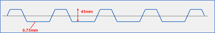
t : thickness of sheeting (in mm)
broof: width of the roof (in mm) (roof dimension parallel to the direction of the panel ribs)
s: spacing between purlins
hw: profile depth of sheeting
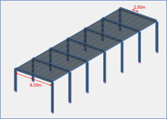
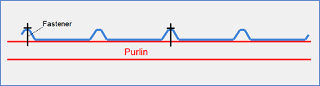
Assume a purlin connected to the following trapezoidal sheeting, at each rib:
Roof width : 6,00m
Distance between purlins : 2,50m
This result sin a shear stiffness of 8361 kN.
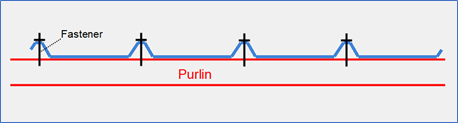
Formula (10.1b) assumes the purlin is connected at each rib to the trapezoidal sheeting :
Purlin connected at each rib
In case the purlin is not connected at each rib but at every other rib, only a small portion (20%) of this S stiffness can be considered :
Purlin connected every other rib
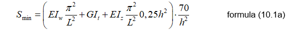
If this value exceeds a certain value (Smin), the purlin may be regarded as laterrally restrained in the plane of the sheeting.
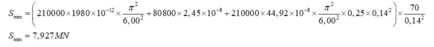
Assume an IPE140 purlin:
Iw = 1980 cm6 (warping constant of the purlin)
It = 2,45 cm4 (torsion constant of the purlin)
Iz = 44,92 cm4 (minor axis inertia of the purlin)
h = 140 mm (height of the purlin)
L = 6,00m (span of the purlin)
In our case, S > Smin. The condition is met and the purlin may be regarded as laterally restrained.
In Advanced Design, such a purlin may have its ‘Continuous restraint along flange’ property enabled on the upper flange :
For more complex cases, when the member is prone to torsional effects (Channel or Z section for example), a more sophisticated calculation may be required (2nd order calculation with warping).
In this case, the shear stiffness (S) may be taken into account as the ‘Shear field’ parameter from the ‘Advanced stability’ dialog :
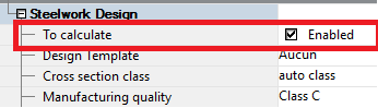
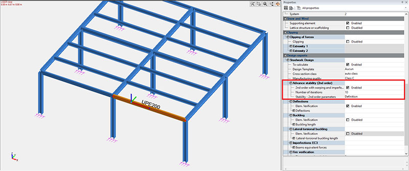
In order to perform second order analysis on steel elements in Advance Design, Steelwork Design “To calculate” option must be activated from the element’s property list.
Figure 1 – Steelwork Design Activation
This feature is available either for each individual steel profile or for a multiple selection, by checking 2nd order with warping and imperfections checkbox, setting the Number of iterations and Stability 2nd order parameters.
Figure 2 – Advance Stability Activation
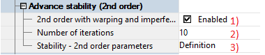
The “Advanced stability (2nd order)” parameters can be found in the Steelwork Design section of the property sheet for steel members.
Figure 3 – Advance Stability Options
(1) Checking the “2nd order with warping and imperfections” box will perform the analysis of the selected members during the steel calculation sequence. (2) The 2nd order analysis being an iterative process , the user can set the maximum number of iterations.
The 2nd order analysis uses the user-defined imperfections in order to determine the final 2nd efforts. The imperfections are applied step by step, incrementally, until the final imperfection defined by the user is achieved. At every iteration, the 2nd order efforts are recalculated starting with the previously calculated efforts. Calculations are made until convergeance – defined as the difference between 2 succesive iterations (automatically managed internally by the solver) – is achieved, or until the maximum number of iterations is achieved.
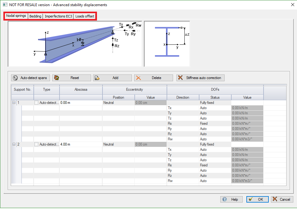
(3) The “Stability – 2nd order parameters” will give access to a dialog where the user can define the various parameters to be considered during the analysis of the selected members. The definition dialog will show 4 tabs: • Nodal springs • Bedding • Imperfections EC3 • Loads offset
Although the “Advanced stability” from Advance Design feature considers the individual member, the intersections with the other elements are of course taken into account. In fact, the intersections are turned into nodal springs.
Figure 1 – Auto Detect Spans Option
The selected member has intersections with other elements at x = 0.00m and x = 4.00m.
The “Auto-detect spans” button enables the users to see the intersections and alter the behavior of the corresponding springs.
The users can also add or delete nodal springs (only user-added nodal springs can be deleted) from the grid using the “Add” and “Delete” buttons. Moreover, they can reset the grid with the help of the “Reset” button.
Note: Even if the user does not open the Advance stability definition parameters, Advance Design will automatically take into consideration the intersections with the other elements during the analysis.
Note: If geometrical parameters are modified after the “Advance Stability” option is checked for steel members, “Reset” and “Auto-Detect Spans” options must be selected in order to reinitialize the position of the nodal springs. Any modifications made in the Advance stability window will be reset to default. Otherwise, the calculation will not be successful.
For each nodal spring, the user can set the status for each of the seven DOF.
Tx, Ty and Tz stand for the displacement along the x, y and z axes respectively
Rx, Ry and Rz stand for the rotation about the x, y and z axes respectively
Rw is the warping
Figure 2 – The seven Degrees of Freedom
Available statuses are:
Free: enables the release for the considered degree-of-freedom ;
Fixed: disables the release for the considered degree-of-freedom (this translates into a very high stiffness);
Auto: lets Advance Design automatically determine whether the degree-of-freedom is free or treated as an elastic release (the stiffness of which is automatically computed by Advance Design for each combination);
Elastic: defines an elastic release for the considered degree-of-freedom (stiffness imposed by user).
When set on “Auto“, Advance Design is able to compute the appropriate stiffness of the release as Force/Displacement, resulting in a stiffness value for each combination.
Figure 3 – Stiffness definition
Warning: the “Auto” status means that the “Advanced stability” feature will attempt to re-create the boundary conditions based on the Forces and Displacements diagrams from the global model.
This can be challenging in some cases as the automatic determination has its own limitations.
For example, zero forces on a given node can either mean:
The degree-of-freedom (DOF) is free;
The DOF is fixed but no force was acting in the given direction.
Therefore, we would advise the users to manually set the free DOF”s on “Free” whenever possible as the “Advanced stability” feature is not able to import the boundary conditions defined on the member in the global model. The “Advanced stability” feature can only deduce the boundary conditions from the Forces and Displacements diagrams it imports from the global model.
We would also advise the users to make sure the member does not feature a free “Rx” DOF on both ends as this could lead to a numerical instability if no other intermediate nodal spring exists.
Setting the “Rx” DOF on “Fixed” can be a solution when the “Auto” detection method fail.
Figure 4 – Degrees of Freedom Status
The “Position” property enables the user to define an eccentric spring.
Eccentricity is meant in the z direction (Upper fiber, Neutral, Bottom fiber or User value).
Figure 5 – Nodal Springs Position Eccentricity
Stiffness auto correction There are cases when, by activating the “Auto-detect spans” option, the automatically calculated stiffness does not meet the minimum criteria in order to successfully perform the 2nd order analysis (for example, when displacements are automatically imposed at an element”s ends for which the automatically calculated stiffness is insufficient). By activating the “Stiffness auto correction” option, the program automatically imposes a minimum stiffness in order to successfully perform the analysis, but only when the values are very small.
Figure 6 – Stiffness Auto Correction Activation
Generally, the warping DOF (degree-of-freedom) is free and fixing it requires special rules for detailing, like the end plates, beam extensions, flat stiffeners.
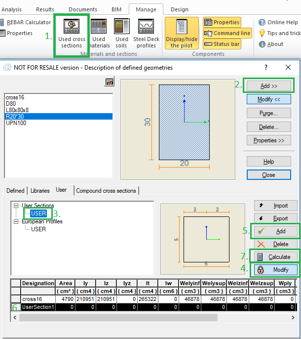
The reinforced concrete linear elements are usually characterized by square, rectangular or circular cross-sections. Advance Design computes the reinforcement for such elements with the Reinforced Concrete (RC) Design expert. For irregular, user defined cross sections, the RC design falls outside the standard procedure. Therefore, the real reinforcement may be determined following an iterative process, as described in the next steps:
1. Add a new user defined cross-section – follow the steps from Figure 1
Figure 1 – Steps to define a new user section
2. Define the cross-section geometry (shape and reinforcement position) and material in the Cross Sections module: draw the shape by point coordinates, define the reinforcement (automatic or manually) and concrete cover, define the material and calculation settings.
Note: It is recommended to define the initial reinforcement from the minimum reinforcement area.
Figure 2 – Define the cross-section shape and place the reinforcement
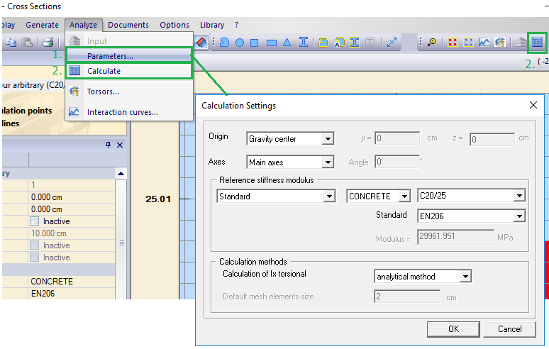
3. Set parameters and calculate the cross-section properties
Figure 3 – Calculation settings
4. Export the cross-section to the Advance Design library
Figure 4 – Close and export the cross-section to Advance Design library
5. The user defined section is attributed to the desired linear elements (columns). Run FEM and RC Design analysis.
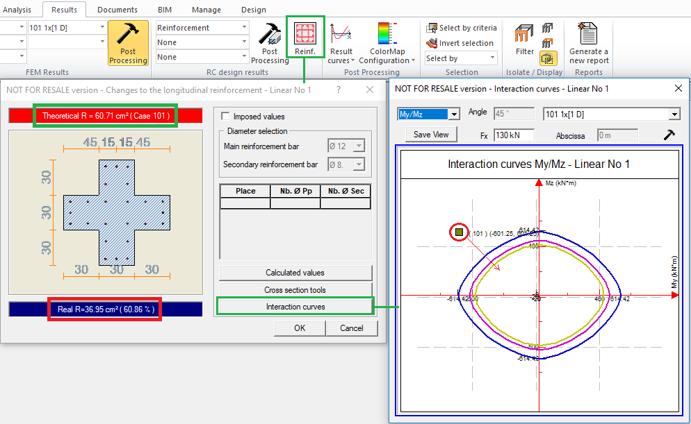
6. On the selected element, check the RC design – element reinforcement results. The real reinforcement (imposed) can be compared to the theoretical reinforcement (computed). The verification can be observed on the interaction curves also. The section solicitation point should fall inside and close to the capacity curve (My/Mz, Fx/My, Fx/Mz), for a safe and economic design. If the imposed reinforcement does not satisfy these conditions, the initial reinforcement is increased: restart from Step 2.
In this short article, we will look at one of the model validation methods available in Advance Design – displaying modelled elements in color according to selected criteria. Although this functionality is more general and can be used simply to improve the way a model is presented in a view or for documentation, today we will focus on its advantages for model verification.
Let us start with the topic of verification of local system of axes of surface elements. Checking and eventual change of local systems is an important step in the verification of the model, because by proper arrangement of local systems we have control over the uniformity of the FEM results and the reinforcement directions. Each modelled planar element has its own local system of axes, which is set automatically. Knowing the basic rules of automatic local axis system setting (as for example that the x-axis of the local system is usually defined along the first edge of the drawn contour) we can often control it ourselves. However, this is not always convenient or possible, especially when the model has been imported. Checking the local layout of axes for one or more elements is not a problem – we can simply select a surface element and we see its local axis symbol by default. The colors of the axes correspond to the colors of axes of the global coordinate system, i.e., the red axis is local x, the green one is local y and the blue one is local z.
However, it is much more interesting how we can quickly check the local axis settings for a larger number of elements / for the whole model. To do this in Advance Design, we can use a very versatile tool to display objects in color according to selected criteria, available in the Display Settings window. In the ‘Color’ command group, there is a list for selecting coloring criteria, as well as additional options including displaying a legend and displaying the element’s local system axis during element selection.
For our purposes, of the many criteria available here, three will be useful to us: Local x orientation, Local y orientation and Local x orientation. All these modes are used to indicate in which direction the axes of the local system are oriented relative to the global system.
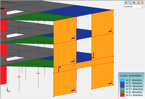
Take a look at the image below showing an example of the effect of using the ‘Local x orientation’ option.
The surface elements are colored and thanks to the legend we can immediately see how the local x-axis is oriented. For example, dark blue means that the local x-axis is pointing in the Y- direction of axis of the global system, light blue means that it is pointing in the Z- direction (down), while red means that it is pointing in the Z+ direction (up). We can easily confirm this just by selecting elements, as then we can see symbols of local systems.
If we now want to unify the orientation of the local axes, all we need to do is select the relevant elements, which is very easy thanks to the colors, and then choose one of the dedicated commands: Local Axis or Local Axis on direction.
On a similar basis, we can verify the orientation of the other axes of the local system of planar elements, but in the same way we can verify the local systems of linear elements. Of course, for this purpose, it is best if we filter out only the linear elements for presentation. But the same types of coloring styles as for surface elements can be used for this purpose.
The layout of local axes is not all that we can verify with coloring. The same tool can be used to verify the correctness of the modeling according to other criteria – for example thicknesses.
On the same principle, we will also check the cross-section of linear elements or the material that has been assigned to different elements of the model. But that’s not all. In a similar way, we can color elements according to their type, system assignment, or super element affiliation. And, other objects, such as loads by category or steel connections by type. I recommend that all Advance Design users become familiar with all the available coloring criteria because using them increases the control over the model.
In order to simulate the membrane effect in a structure in Advance Design, “DOF (Degree of freedom) constraint” object can be used with the Tx and Ty translations restrained. DOF constraint object is also named as Master-Slave connection. The command can be found in “Objects” ribbon tab:
Figure 1 – DOF constraint localization
The following properties regarding restraints definition are defined for the “DOF constraint” (Master-Slave connection):
Figure 2 – DOF constraint properties
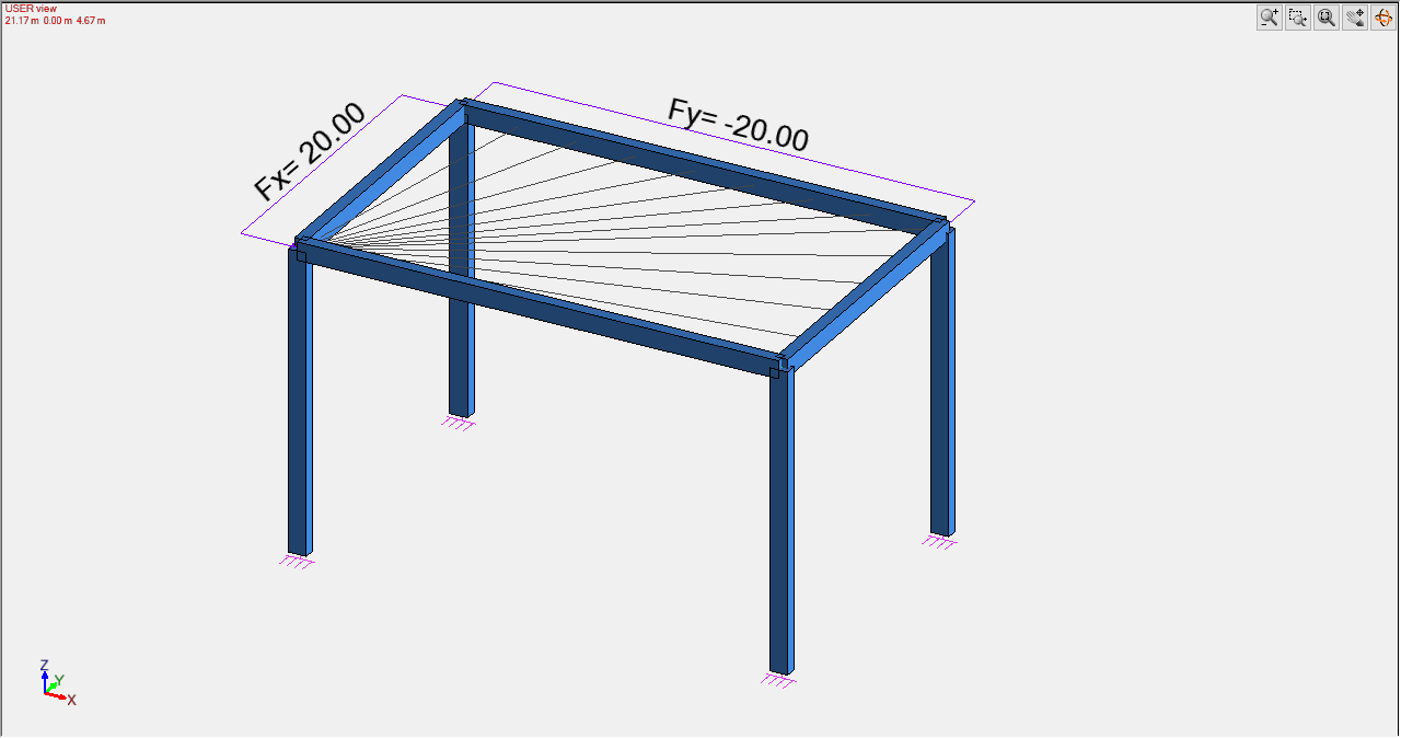
For example, the response of the DOF constraint is compared with the response of a membrane in a simple 3D structure subjected to lateral loads. In this model, the elements’ self-weight is not considered.
Figure 3 – DOF constraint model view
Figure 4 – Membrane model view
Since the master-slave connection imposes to all component nodes the same DOF restraints (translations/rotations), the master node can be placed anywhere on the perimeter. In order to simulate the same response, the nodes must be placed on the same position as the mesh nodes of the membrane:
Figure 5 – DOF constraint mesh view
Figure 6 – Membrane mesh view
The similar response of the two objects (master slave connection with Tx and Ty translations restrained and membrane) can be verified by comparing the results of the FEM analysis:
Figure 7 – Displacements comparison between the two models
Figure 8 – Axial force comparison between the two models Figure 9 – Bending moments on columns comparison between the two models Figure 10 – Bending moments on beams comparison between the two models
BIM WORKFLOW WEEK is an online event organized by GRAITEC for structural engineers and detailers. Nowadays, you can streamline your BIM workflows using Graitec and Autodesk technologies together. Bridge the gap between all stakeholders and discover how you can develop and improve your construction projects in a digital thread!
Each day we will run a webinar to show how easy it is to streamline your daily work! We show how to apply a complete BIM workflow from design to detailing on all your projects during the webinars! Don’t wait and register today!
BIM WORKFLOW WEEK AGENDA:
Monday – 15/03/2021 – CREATE YOUR BIM MODELS WITH REVIT AND SIMULATE THEM WITH ADVANCE DESIGN
Are you a structural engineering company doing construction projects with Revit® from Autodesk in a BIM environment? In this webinar, we will propose you a way to streamline your projects, starting to CREATE BIM data in Revit, exporting it to Advance Design to SIMULATE your building and synchronize back in Revit all changes. Discover how easy it is to link Autodesk Revit and Graitec Advance design to simulate and optimize your steel an concrete projects.
Tuesday – 16/03/2021 – ENRICH YOUR 3D BIM REVIT MODEL WITH ANALYTICAL DATA AND RESULTS USING ADVANCE DESIGN
In this webinar, we will go deeper in the integration between Autodesk Revit and Advance Design: exchanging and synchronizing geometrical data is a good point but is not enough to enable a real BIM structural workflow. During this session, you will discover how to enrich your Revit model with finite element results and theoretical reinforcement values using Advance Design with an effective synchronisation mechanism controlled by the user!
Wednesday – 17/03/2021 – APPLY AN EFFECTIVE BIM WORKFLOW FOR ALL YOUR REBAR PROJECTS IN REVIT!
In this BIM era, it’s time for you to manage your rebar projects with 3D models using Autodesk Revit®! Join us to this webinar and discover how you can use the Autodesk platform and Advance Design together to produce 3D Design-driven rebar cages for Beams-Columns-Footings-Slabs-Walls & Shear Walls, automate the drawing views creation with all tags and annotations, produce final drawings and manage in real time all your rebar projects!
If you’re a structural engineer or a steel detailer using Advance Steel and want to save time, cost and reduce your carbon footprint, Graitec now offers a solution to complement and optimise your current workflow. To facilitate analysing these complex 3D steel connections, Advance Steel joints can now be exported to Graitec Advance Design Connection!
Friday – 19/03/2021 – APPLY A COMPLETE BIM WORKFLOWS FROM DESIGN TO DETAILING ON ALL YOUR STEEL PROJECTS!
In this webinar, we will go through a complete BIM workflow from design to detailing using Autodesk Advance Steel and Graitec Advance Design together. You will discover how easy it is to design and optimise a steel structure with Graitec Advance Design, including steel joints. Then, we will end by exporting the model to Advance steel to create drawings, BOM lists and CNC files fir the fabrication.
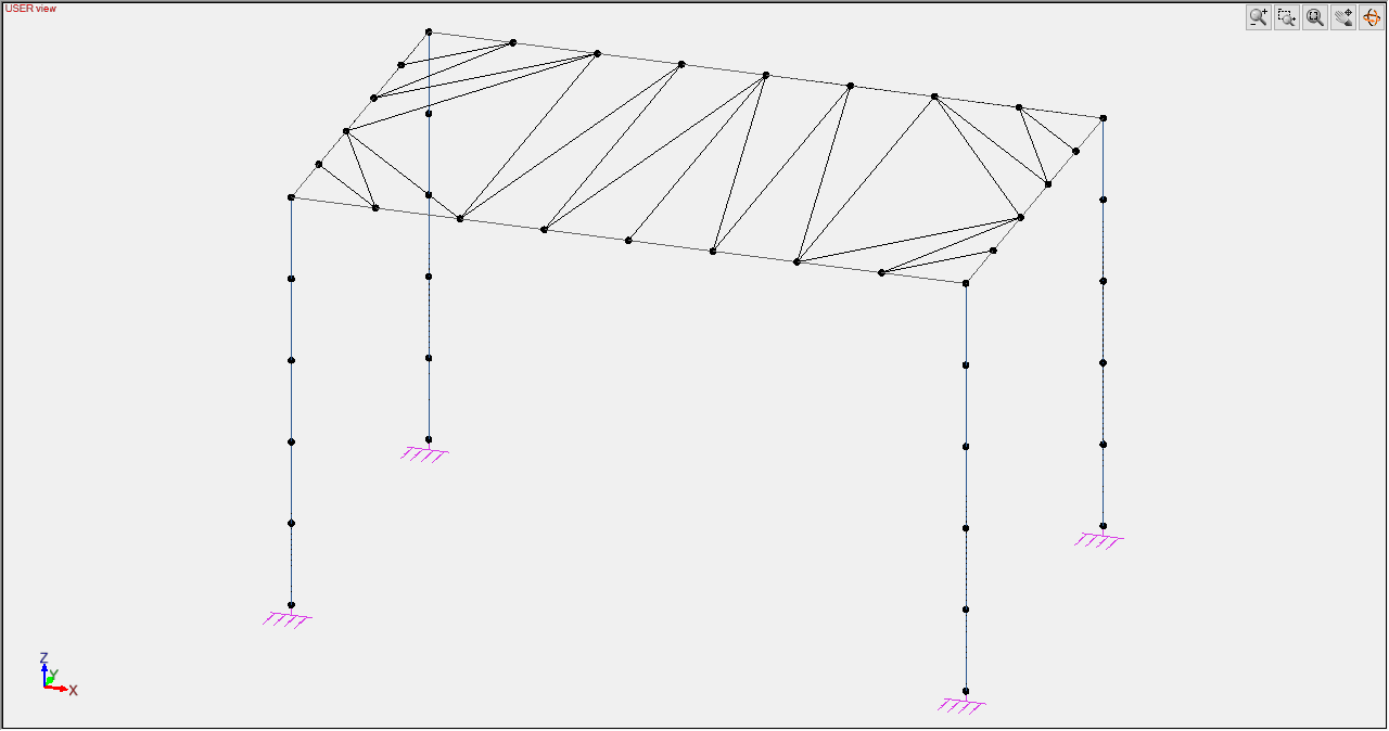
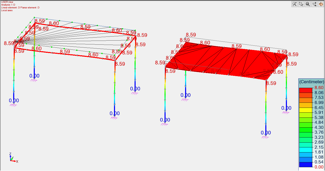
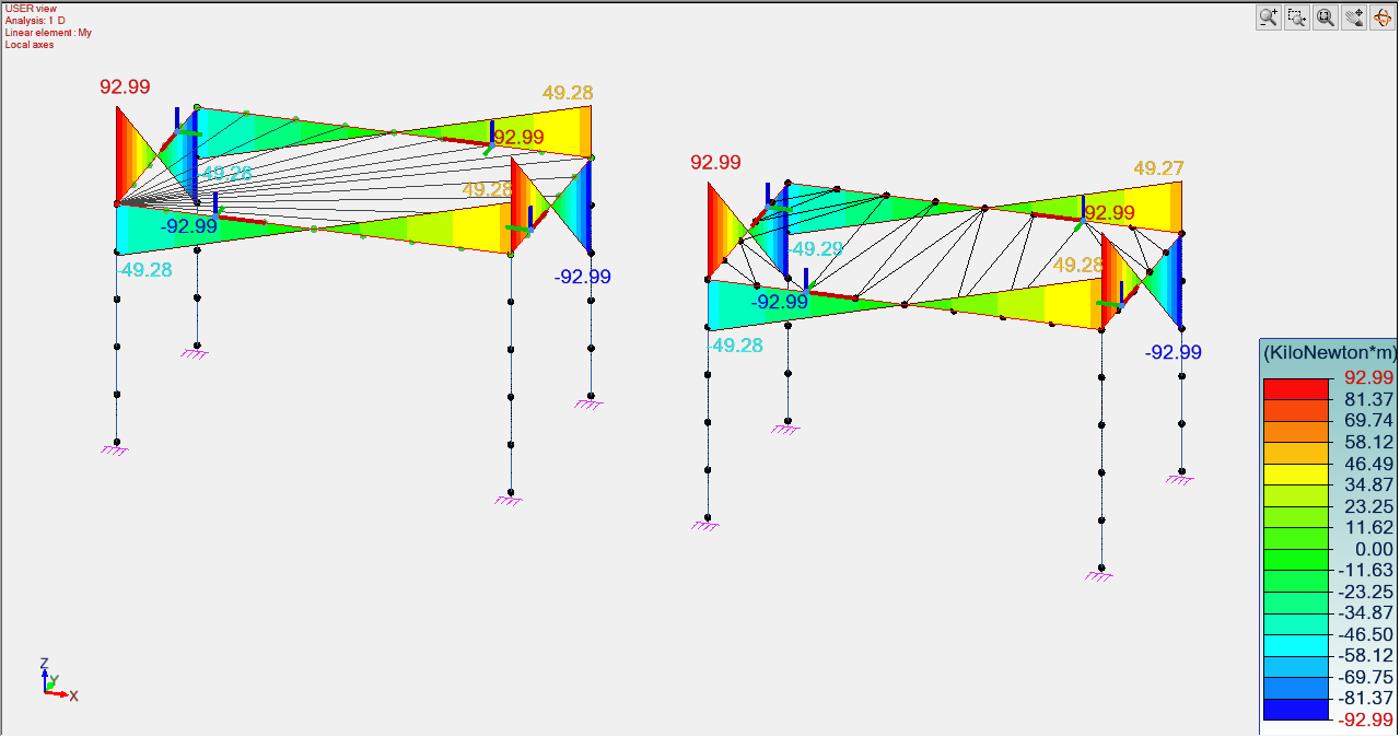
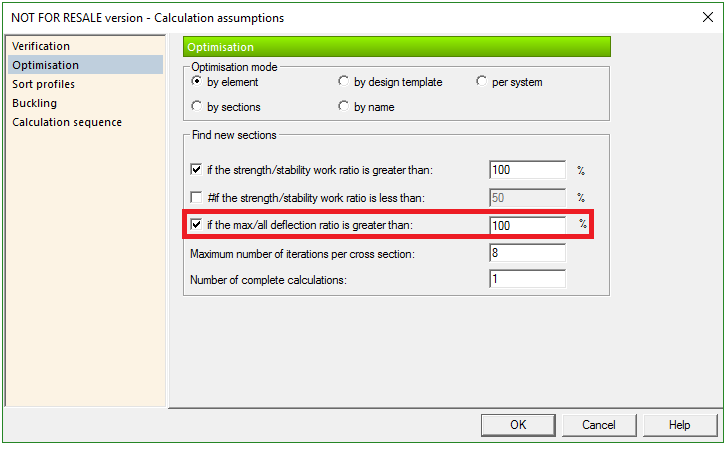
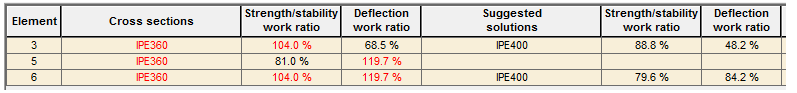
The shape optimization calculation for steel elements can be performed in Advance Design considering the condition of maximum deflection. Then, new cross-sections are searched if the deflection ratio is greater than the set limit (default 100%).
Thanks to this option from Advance Design, it is possible to optimize steel elements while using more criteria at the same time, like searching and selecting for profiles that must meet the conditions for maximum load capacity (strength/stability) and maximum deflection, independently or at the same time. This is especially useful for design of steel structural elements that exceed the maximum deflection while meeting the load capacity condition.
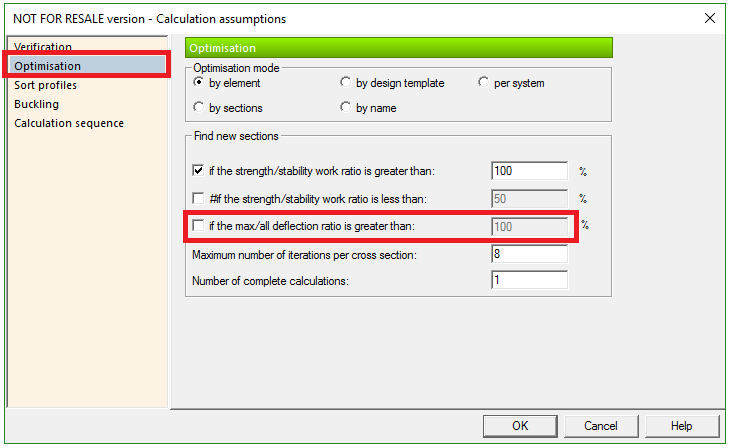
The optimization assumptions can be found in the Optimisation tab from Steel Design Calculation Assumptions dialog. Under the “Find new sections” paragraph, a new option is available to activate the deflection criterion and to set the maximum allowable deflection ratio considered for the cross section optimization. These assumptions apply to all steel members from the model which have Steelwork DeDefault optimization assumptionssign option from the element’s properties activated. The limits imposed in this tab apply to all cross sections as a group and cannot be applied differentially for singular element.
By default, the deflection ratio optimization is unchecked:
Figure 1 – Default optimization assumptions
By checking the “if the max/all deflection ratio is greater than:” option, the user can impose the maximum ratio.
Figure 2 – Activation of the deflection optimization criterion
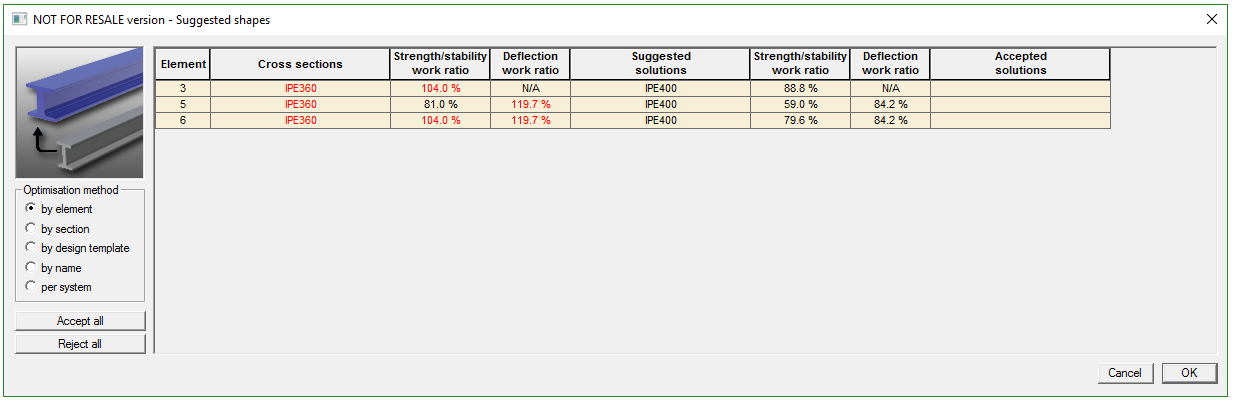
Once the steel calculation is completed, the strength/stability and deflection work ratios of steel elements are compared with the specific criterion, and other cross sections that meet the imposed conditions are suggested. The results of steel elements optimization are displayed in the Suggested shapes dialog, displaying the current strength/stability and deflection ratios. If the ratios are greater than the imposed limits (100% by default), the current ratio is displayed in red. For such cases, if the deflection criterion is activated, the next cross section from the catalog that will meet the required criterion will be suggested, displaying also the ratio for that section.
Figure 3 – Suggested shapes according to selected criterion
By opening the Accepted solutions flyout, we can select the suggested shape or other section from the same catalog.
Figure 4 – Selection of accepted solutions
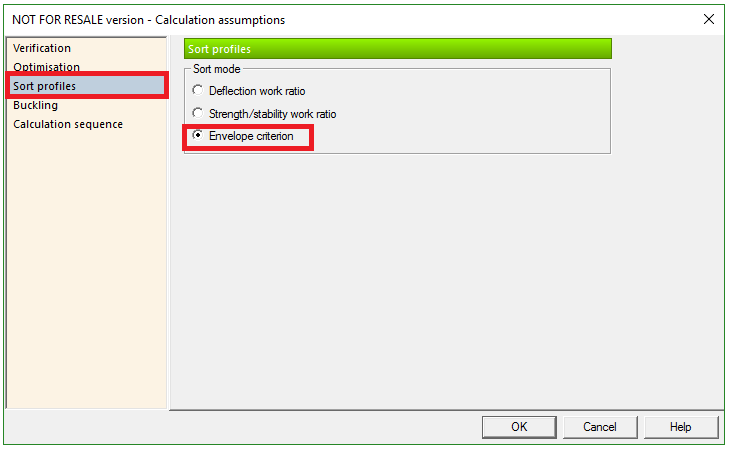
After accepting the suggested (or imposed) sections, from the Accept all option, a new steel calculation is required, in order to recalculate the new sections and have correct results in the shape-sheet of the elements and reports. This optimization sequence is directly dependent with the sorting mode selected in the Sort profiles tab from steel Calculation assumptions. By default, the “Envelope criterion” option is selected, which means that the suggested profiles will meet both deflection criterion and strength/stability criterion.
Figure 5 – Default sort mode for section optimization
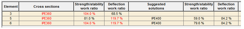
If the Envelope criterion is selected, the new profiles are suggested from both cases, if the deflection or strength/stability criterion are exceeded:
Figure 6 – Suggested shapes according to envelope criterion
If the Deflection criterion is selected, then the new profiles are suggested only if the deflection ratio is exceeded:
Figure 7 – Suggested shapes according to deflection criterion
If the Strength/stability criterion is selected, then the new profiles are suggested only if the deflection ratio is exceeded:
Figure 8 – Suggested shapes according to strength/stability criterion
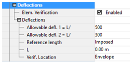
In order for the deflection criterion based optimization to be computed, both Steelwork Design and Deflections options from element’s property list must be checked. The optimization based on deflection will be made according to the parameters introduced in the property list:
Figure 9 – Element property check
If the deflection verification is unchecked for an element, then “N/A” (Not available) message will be displayed for the Deflection work ratio in the Suggested shapes dialog.
This new feature makes result checking easier, thanks to the possibility of presenting a ratio for deflection during shape optimization. It also gives you the possibility to select optimal steel profiles considering the deflection. Various options from the Assumptions dialog help you get specific results for the steel elements used in design and enhance the workflow.
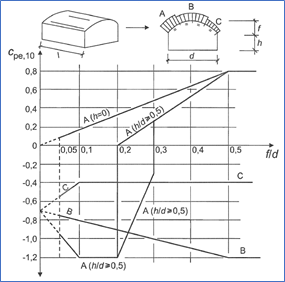
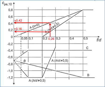
The present article explains how to determine wind loads on vaulted roofs at the Eurocode 1. Specifically, we will show how to use Figure 7.11 from EN1991-1-4, which provides the external pressure coefficients on vaulted roofs with rectangular base:
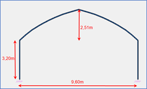
We will consider a structure with following dimensions:
f = 2,51m
h = 3,20m
d = 9,60m
The developed length of the vaulted roof will be split into 4 equal parts, for zone A, zone B (repeated twice) and zone C:
For each of these zones, the external pressure coefficient (Cpe10) is read on a graph, depending on the f/d and h/d ratios.
In our case:
f/d = 2,51 / 9,60 = 0,26
h/d = 3,20 / 9,60 = 0,33
For zone A
We start on the f/d axis until we reach the two diagrams related to zone A:
For h/d = 0, we read Cpe10,A = +0,42
For h/d ≥ 0,5, we read Cpe10,A = +0,16
We then perform a linear interpolation because in our case, 0 ≤ h/d ≤ 0,5:
For h/d = 0,33, we get: Cpe10,A = +0,25
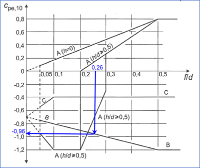
For zone B
We start on the same position on f/d axis, but this time, we reach the zone B diagram.
We read: Cpe10,B = -0,96
For zone C
We read: Cpe10,C = -0,40
In the end:
For zone A => Cpe10,A = +0,25
For zone B => Cpe10,B = -0,96
For zone C => Cpe10,C = -0,40
Starting from version 2021, vaulted roofs at the Eurocode 1 are covered by the climatic generator of Advance Design.
Wind actions, whether 2D or 3D, are instantly generated:
As prescribed in the Eurocde 1, roof is divided into 4 equal zones.
The name of each zone as well as their Cpe value can even be displayed with a dedicated annotation:
Conclusion
The evaluation of wind action on vaulted roofs by reading the graph from the Eurocode 1 can be tedious, with a high risk of error.
Fortunately, in Advance Design, this process is fully automated. Wind forces are created instantly, and they can be updated in a single click whenever a modification is made on the building.
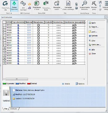
The calculated structure can be synchronised with the Revit input model; to do this you export the model from Graitrec’s structural analysis software, Advance Design, using BIM Connect. Then select the synchronisation option in Revit and indicate the location of the exported file. The software generates a list of all elements, creating a breakdown of added, changed and deleted elements.
After reviewing the changes that have occurred in relation to the calculation, you can accept, ignore or remove the changes from the sync list. Once the changes are accepted, the model in Autodesk Revit will update.
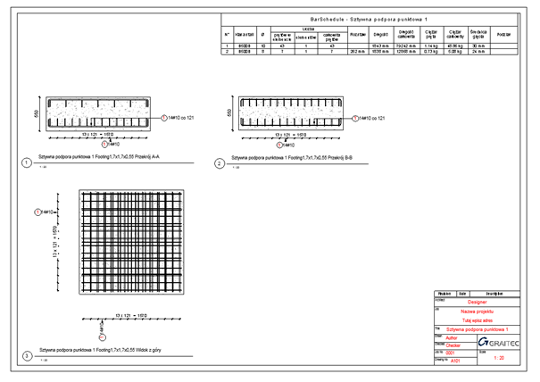
In Revit, using the PowerPack Design module, it is also possible to design foundations together with the calculation of the reinforcement, based on given conditions. After the calculations, reinforcement drawings can be generated automatically. Most of the drawing’s components such as sections, their location, used labels, dimension lines or lists/bar schedules can be saved by the user in a template which is a native Revit file. From this, PowerPack will generate the drawings.
It remains to define the steel connections. This can be done directly in Revit or using Dynamo, but for the sake of shop drawings, it is suggested to export the model to Advance Steel. The connection calculations themselves can be carried out in Advance Design structural analysis software, using the Steel Connection Designer module.
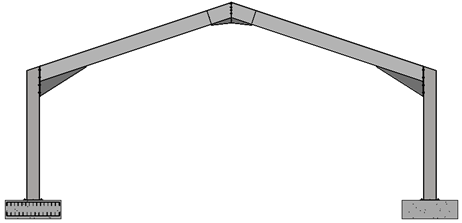
Monolithic floor slabs are currently one of the most popular solutions. Depending on the structural system used, they can cover relatively large spans.
In most cases, the slabs are reinforced with a two-way orthogonal grid up and down. A common misconception among designers is that the determination of the cross-sectional area of this reinforcement for the ultimate limit state is based solely on the bending moments which are the same for the directions of the reinforcement. Thus the dimensioning of the reinforcement in direction “x” would be based on the bending moment Myy and the reinforcement “y” on the moment Mxx.
The example of a simple two-span slab, in which one span operates in a decidedly unidirectional manner and the other in a bidirectional manner, shows how to determine the authoritative, dimensioning moments. The loads and geometry are not particularly relevant. We will mainly discuss the nature of the plate work without attaching importance to values. The model and calculations were made with Graitec Advance Design.
It must be remembered that the orthogonal reinforcement grid results from a certain compromise between its optimality from the load-bearing point of view and the ease of subsequent execution on site. In reality the directions of the principal moments can be and in many places are deviated from the direction of the moment Mxx or Myy. Therefore, the most optimal reinforcement would be one designed according to the trajectory and based on the values of the principal moments M1 and M2.
Remember that the values of the principal moments must be interpreted with their directions, since they are not local or global values of the structure. Where the principal directions coincide with the directions of our reinforcement, i.e. x and y, this means that the dimensioning value of the bending moment will be the moments Mxx and Myy and the trajectory of this reinforcement is the best possible.
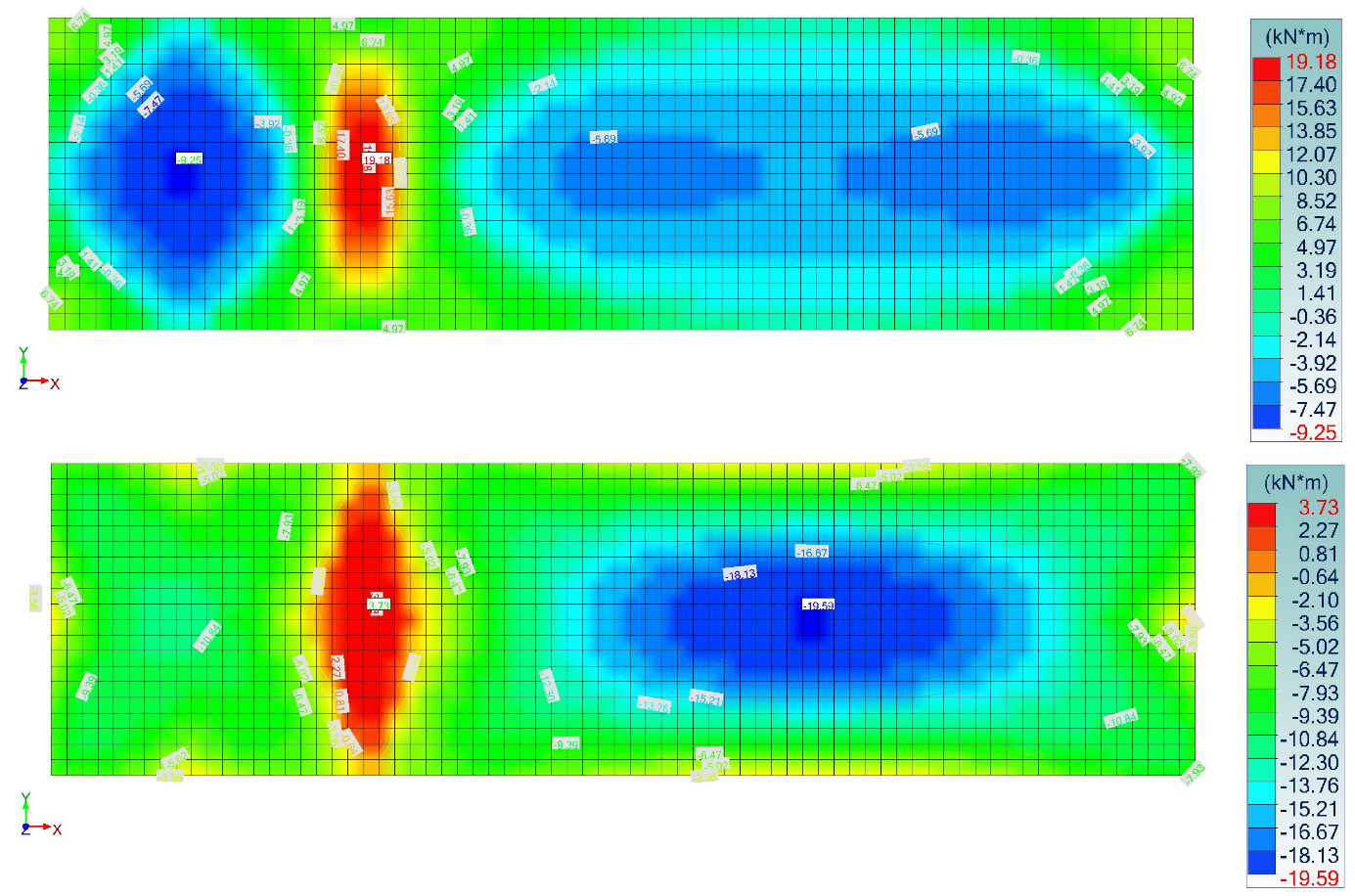
It is easy to see that the directions of the principal moments coincide with the x/y direction in the central bands, but deviate at the corners. Most designers who have ever dimensioned slab reinforcement in more sophisticated FEA-based software have probably noticed that the reinforcement map does not correlate directly with the maps of orthogonal bending moments in the local floor system.
The “butterfly” shape of the two-way free-supporting slab and the top reinforcement of the corners in both the X and Y directions are very characteristic. This is usually the most questionable aspect for designers – after all, the bending moment maps in no way correspond to this distribution of reinforcement – but it is perfectly normal behaviour.
The devil is in the torsional moment Mxy/Myx. Its presence is responsible for the deviation of the moments from the x/y direction. In the main directions we are only talking about the moment M1 and M2, there is of course no torsional moment there. If you decide to deviate from the main trajectory and reinforce the slab with orthogonal mesh, you must take this moment into account in the dimensioning of the reinforcement. The program Advance Design does this automatically of course by determining the relevant dimensioning moment at each grid point. In short, this means the projection of the principal moments onto the reinforcement directions.
Influence of dimensioning forces on the dimensioning of reinforced concrete
When dimensioning reinforced concrete members, the program determines the dimensioning forces which the user can display on the structure at any time.
Literature on the principles of reinforcement design for reinforced concrete slabs recommended the use of bottom diagonal reinforcement in the corners of free-supported slabs with a certain cross-sectional area (most often referred to as maximum span reinforcement in this literature). Designers usually use such reinforcement, but often without being aware of the design necessity. It is important to realize that the above-designed orthogonal X/Y reinforcement taking into account the torsional moment closes the topic and we are not required to use any additional reinforcement with a trajectory separate from the orthogonal reinforcement. The fact remains, however, that orthogonal reinforcement is not fully optimal.
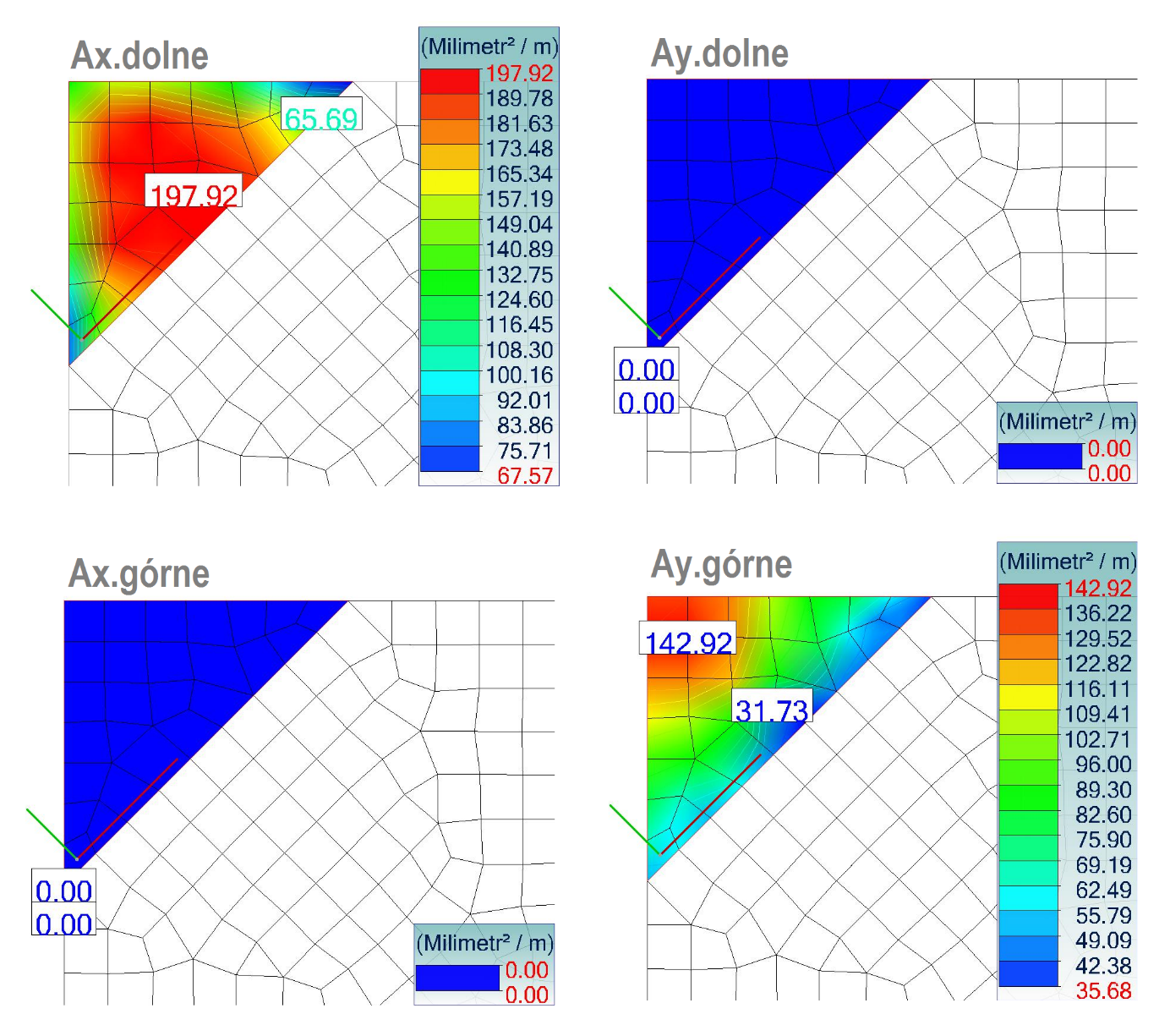
To illustrate this phenomenon, it has been decided to model in the corner a slab whose local directions (and thus also the directions of the reinforcement in the adopted settings) are in accordance with the directions of the principal moments.
When using orthogonal reinforcement, both top and bottom reinforcement in both X/Y directions were required. For trajectory reinforcement, a bottom reinforcement perpendicular to the bisector and an upper reinforcement parallel to the bisector is sufficient. This means that the principal moments are at this point deviated by 45º from the X/Y direction.