Abstract

In this article, you will learn about the possibilities of Advance Design for the graphical presentation of results for surface elements.

Keywords: Advance Design, Finite Elements, FEM, Floors, Slabs, Walls

Graphical presentation of results for surface elements

Advance Design can generate and calculate various types of three-dimensional structures, including those containing flat surface elements (such as slabs or walls), as well as shell elements (e.g. curved roofs or circular tanks). In addition to the preparation of the model and the execution of the calculations, an integral part of the design process is the review, evaluation, and documentation of the calculation results. Today we will look at one aspect of this – the ways in which results for surface elements are presented graphically in Advance Design.

Model

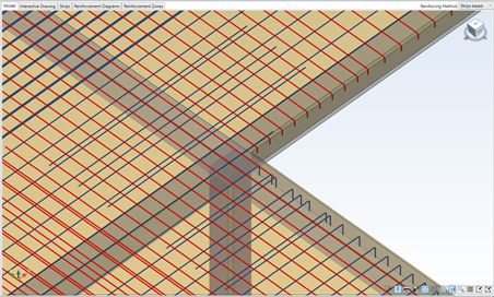
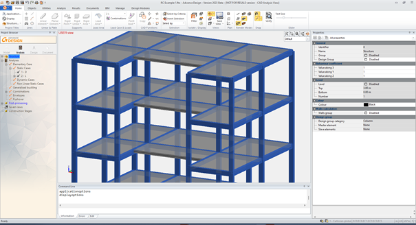
The available methods will be presented on the example of one slab of a very simple spatial model of a concrete structure.

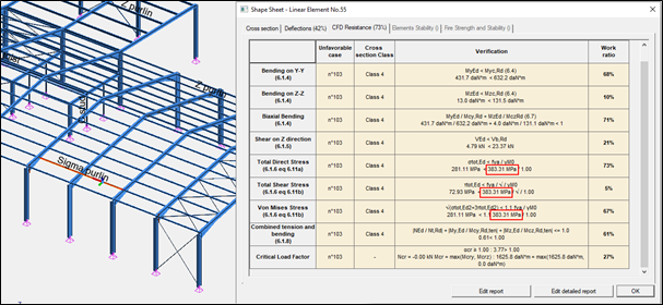
For the selected load case, we will check the graphical presentation of the displacement results, but the same methods as presented below can be used to display other types of results, ranging from internal forces and stresses to outputs related to the design of reinforcement (for example reinforcement areas or crack values).

How to change display settings for results

With the model calculated, displacements for all or selected part of the model can be displayed directly using the commands available on the ribbon. The results are then presented using a default display mode – in the case of displacements this is called ‘Deformed’. To change the mode, use the window with the setting of graphic results (opened, for example, using the keyboard shortcut Alt+Z). Note that the list of available display modes depends on the type of element and the type of result. In the case of surface elements, a list as shown in the image below will be available.

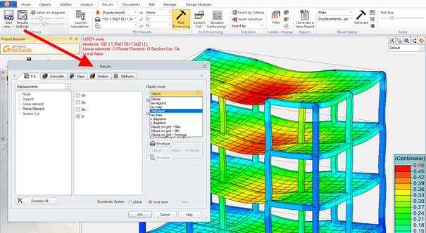
Available display modes

Let’s now take a look at the display modes available. The default one is called ‘Deformed’ which presents the results as color maps on the deformed structure. This mode is available also to linear elements, which allows showing results for a whole structure using common color scale.

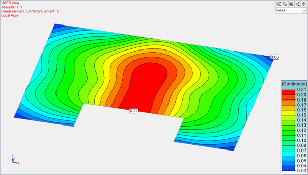
There is a twin mode, called ‘Iso regions’, which also shows the results as maps but only for surface elements. The iso-value regions represent colored polygons on the planar elements corresponding to certain results on displacements, forces, stresses. Thus it is possible to view the highest stress areas on the planar element within a single glance. The values of these regions can be smoothed or not; for this purpose you can use the option “Smooth results on planar elements” from the Results dialog box – Options tab.

The next display mode is called ‘Iso lines’. The color of iso lines correspond to the results color scale. Note that regardless of the selected style, additional presentation options can be set, such as visibility of the finite element mesh, display of extreme values or values corresponding to particular iso lines.

The next display mode is called ‘Iso maps’, which combines the display of isolines and solid color maps.

As mentioned earlier, we can control additional graphical settings. In the example below, we have the same display mode but with isolines turned off and values displayed in finite element centers.

The next two similar display modes are called ‘X Diagram’ and ‘Y Diagram’. These are diagrams in the X or Y direction of the local system respectively, displayed in a plane perpendicular to the surface element. As these diagrams pass through the centers of the finite elements the resulting effect depends on the density and shape of the mesh.

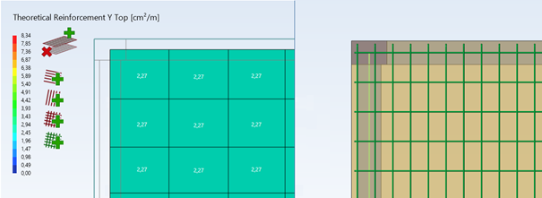
The next display mode available is called ‘Values’. And as the name suggests, it displays values in finite element centers. Depending on the settings the values can be displayed in scale colors or in solid color.

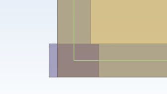
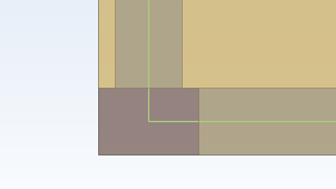
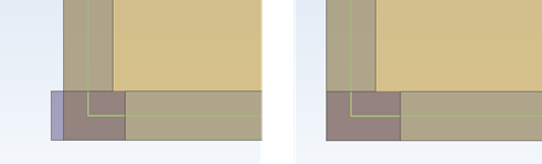
As the values can be difficult to read (too small or overlapping) in the case of a dense or irregular finite element mesh or at lower magnification, we can display the values using another style called ‘Values on grid’. This display mode comes in three variations – for presenting minimum, maximum or average values in a grid. The results grid is a virtual mesh of regularly arranged rectangles used only for the presentation of results.  The setting of the mesh size is available individually in the properties of each surface element.

Additional settings

In addition to the presentation display modes, Advance Design offers various additional options for setting the presentation of the results. Firstly, we can control the color scale. For example, we can set a reduced number of ranges with defined limit values.

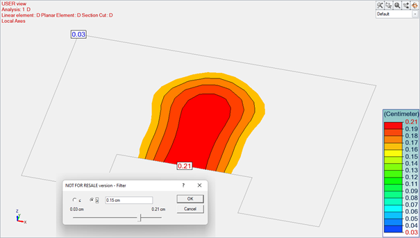
Another possibility is the presentation of results using Dynamic Contouring command. This allows you to filter the displayed values to a selected range.

Another way of presenting results for surface elements is to display intersection diagrams. These are created using linear Section cut objects. You may create section cuts in the modeling step and in the analysis step, and like all elements of the model, the section cuts may be selected, resized, moved using CAD tools. Diagrams on section cuts may be generated in the element plane or in a perpendicular plane.

Finally, it is still worth mentioning that for planar elements it is possible to view the forces and stresses results expressed in the main axes. For this we use dedicated display mode called ‘Main axes’. The two main axes are represented graphically by their color, the sign is represented graphically by the arrowhead direction (inward for negative values and outward for positive values) while the angle of axis orientation is given by the alpha values.

Learn more about Advance Design!

Visit website – https://graitec.com/advance-design/
Visit Advance Design Virtual Stand – https://graitec.com/advance-design-virtual/
Linkedin – https://www.linkedin.com/showcase/advance-design-&-advance-design-connection/
Free trial – https://graitec.com/free-trial/

Abstract

In this article, we will follow the rules from EN1996-1-1 to verify an unreinforced masonry wall subjected to an in-plane lateral force.

Keywords: Advance Design, Masonry, Eurocode 6, EN1996-1-1

1.     Introduction

Masonry can effectively carry compressive forces but this material only has moderate capacity when it comes to shear.

Yet, masonry walls may be exposed to wind forces that could cause shear failure mechanisms, especially on the top levels, where the compressive forces are moderate.

Therefore, shear resistance of masonry walls must be properly assessed.

Eurocode 6 provides a method in that regard.

2.     Sliding shear resistance of an unreinforced masonry wall

Unreinforced masonry walls subjected to shear loading are covered in section 6.2 from EN1996-1-1.

As usual with the Eurocodes, a design force (V_Ed, design shear force) is compared to a resisting force (V_Rd, shear resistance).  

2.1.            Assumptions

Assume the following wall:

Material characteristics

Initial shear strength: f_vk0 = 0,20 MPa

Compressive strength: f_k = 5,00 MPa

Partial factor for material: γ_M = 2,2

2.2.            Shear resistance V_Rd

Shear resistance V_Rd is defined in eq. (6.13).

First of all, we need to estimate the compressed length of the wall (l_c).

The V_Ed lateral force is indeed creating an in-plane moment that can cause tension at the bottom part of the wall, especially if the compressive forces are low.

• Moment at the bottom of the wall

• Eccentricity

• Compressed length l_c

The eccentricity exceeds 1/6 of wall length.

Assuming a linear distribution and based on the equilibrium of force and moment:

We can assess the length of the compressed part of the wall:

• Shear strength f_vd

Assuming all joints (vertical and horizontal) are filled with mortar, we compute the characteristic shear strength f_vk with eq.(3.5).

The design compressive stress σ_d can slightly increase f_vk.

f_vk does not exceed

The design shear strength is then given by:

• Shear resistance V_Rd

We can finally compute shear resistance V_Rd from eq. (6.13):

Sliding shear verification:

The sliding shear verification is passed.

3.     Conslusion

This verification can prevent some of the shear failure mechanisms that may occur in masonry buildings.

Of course, hand calculation might be tedious.

Fortunately, our upcoming Advance Design module, dedicated to masonry wall design, will perform this verification, among others, in a matter of seconds and provide a detailed calculation report, with intermediate values and reference to the EN1996-1-1.

• Visit website – https://graitec.com/advance-design/
• Visit Advance Design Virtual Stand – https://graitec.com/advance-design-virtual/
• Linkedin – https://www.linkedin.com/showcase/advance-design-&-advance-design-connection/
• Free trial – https://graitec.com/free-trial/

Abstract 

In this article you will see how to define a multi-span concrete beam in Advance Design in order to design and detail it using RC Modules. 

Keywords: #AdvanceDesign #Concrete #Reinforcement 

1. Defining beams in Advance Design 

In Advance Design you can model very different types of objects including planar and linear elements, which will represent our structural elements such as beams, columns, walls and slabs. With defining right section and material we can simulate behavior of our structure using FEM analysis. 

If it comes to concrete beams we always could provide linear element stretching from one support to another. If we defined also intermediate supports like columns or walls our beam would be treated as multi-span. 

2.     Super-element concept for RC design

Even though we could easily design a beam shown on figure 1 above this approach has some limitations. Because it’s a single element we can for example specify only one section height for all spans. However, sometimes we need for a different spans to have different sections due to capacity requirements or some technical aspects (such as need of clear height of a story, leaving some space for ducts and so on).

Starting with Advance Design 2022 it is possible to use super element concept also for RC design. Initially it was implemented for steel structures, however using this workflow was found effective also for other materials.

2.1. Creating a super element in Advance Design

To create a super element we model each span of a beam as a single element. Remember to always define them from support to support. If possible, try keep local axes in the same direction and orientation.

Last thing to do is to convert these 3 single linear elements into one super element. We can do that using context menu at right mouse button or finding these exact options on Objects ribbon.

Note that now you can pick whole super element by selecting any part of it. However if you need to select only a single span for example to change its section you need to toggle pick mode from super elements to elements. You can do it by pressing ALT+E or again find it at right mouse button context menu.

After defining a super element you can see it has now new own identifier, a list of elements which you can always edit if needed and also each element included in this group gets a postscript to its name informing user it’s a super element. Remember you can always cancel super element similar way you created one.

2.1. Design of multi-span beam defined as super element

When you are done preparing super elements, rest is as usual. We need to perform a FEM analysis calculations to obtain static results. Now we are ready to open a super element using RC Beam Module.

Notice that super element shown below has 3 spans of 3 different sections height.

Right now we need to specify requested reinforcement and design assumptions. Element will be designed as it was continuous multi-span beam. Reinforcement drawings and schedules also can be provided for whole element at once.

• Visit website – https://graitec.com/advance-design/
• Visit Advance Design Virtual Stand – https://graitec.com/advance-design-virtual/
• Linkedin – https://www.linkedin.com/showcase/advance-design-&-advance-design-connection/
• Free trial – https://graitec.com/free-trial/

Abstract

In this article, you will learn how to start modifying and defining your own drawing style template in Advance Design modules.

Keywords: Drawings, Advance Design Modules, Bar schedules, Templates

Modifying Drawings in Advance Design Modules

The reinforcement drawings generated by Advance Design modules are highly customizable. The range of possibilities is very large and can be divided into two groups – the current modifications that can be done to the generated drawing and the modifications to the templates used for generating the drawings

Current modifications to the drawing are mainly done graphically or using a series of simple commands available from the properties list. Among these are ability to modify the scale, change the position of views on the sheet, add/remove views (as new sections), rename views, add dimension lines, move descriptions or symbols.

The second group of modifications relates to the templates used for the generation of the drawings. There are many different types of templates available, starting from the most general Drawing Style, which is a template collecting all settings and layouts of views, through templates controlling the settings of colors, lines and symbols used, templates for title blocks and templates for rebar lists.

Today we will look at modifying the general drawing template – the Drawing Style.

Drawing Style – general information

 The style template is the most general template and contains a complete description of the drawing, i.e. the orientation of the paper, how many and which views you see, their scale and position on the sheet, used drawing templates, title blocks and bar schedules.

Each module (e.g. RC Beam, RC Forting, …) has its own set of style templates and their number and content is different depending on the regional settings of the program. So drawings may look different according to the default templates for France and the UK for example. However, anyone can easily modify existing templates or add their own.

Changing Drawing Style

Let’s start with how to apply a style other than the default template. The easiest method is to right-click on the first item in the tree (Drawings) and select one of the styles from the available list – Apply Style.

The list shows the styles available in the default styles folder for the given element type and for regional settings (country). By selecting ‘Select styles’ you can preview the contents of the folder and select a file from another location. This command menu also includes a Save Style command that saves all current drawing settings to a new Style template file.

Layout of views

Most of the changes to the settings in the property list (including the sheet format or the type of reinforcement list) as well as the number and type of views are written directly to the template. However, the placement of views and their scale depend on the Layout of views settings. So it is usually not enough to move the contents of a view (for example, a beam cross-section) to a new location on the sheet, but to move its associated rectangular outline, which is presented as a blue frame.  Namely, modify the layout of the views on the sheet  

To check and modify the layout of the views in the current drawing, right-click and select Edit Layout command.

We will then see the layout of the views, which we can freely arrange on the sheet by moving the corners of the outlines (using grips). This will allow us to ‘anchor’ a given view on the sheet, also in relation to the other views.

By default, the views are generated according to the position of the layout frame as well as their scale is automatically adjusted to its size. But we can change these settings using two options from the view properties.

The ‘Views fit layout’ option is responsible for automatically scaling the view so that it fits optimally in the frame area. If you disable this option, the scale will not be automatically modified when regenerating the drawing.

The ‘Views follow layout’ option is responsible for the location of the view relative to the frame area. If you disable this option, the view will not automatically follow the frame area when the drawing is regenerated, i.e. the last position of the view after it was manually modified will be preserved.

The above description, of course, only briefly introduces the subject of template customization, so I recommend exploring the available options on your own. At the end, one more note – remember that the final effect, i.e. finally generated drawings, can also be saved directly in DWG format, allowing further changes or assembling drawings in CAD if necessary.

Learn more about Advance Design!

• Visit website – https://graitec.com/advance-design/
• Visit Advance Design Virtual Stand – https://graitec.com/advance-design-virtual/
• Linkedin – https://www.linkedin.com/showcase/advance-design-&-advance-design-connection/
• Free trial – https://graitec.com/free-trial/

Steel beams supporting a concrete slab are quite common in building practice.

Yet, one might need to determine the equivalent characteristics of the whole system (for quick assessment of dynamic behaviour for example).

This can be achieved manually or with a section editor program.

Let’s consider the system below:

The distance between the centres of gravity is 14cm + 4cm = 18cm:

Modelling in Advance Design

In Advance Design, this result could easily be achieved by using the Section Editor:

First, a rectangular contour is introduced, with concrete material, to account for the slab:

Then, the HEB280 profile is called from the library and positioned right below the slab:

In the calculation settings, we select the intended material for the equivalent member:

Learn more about Advance Design!

For the Base Plate and Tubular Base Plate joints, designed with Advance Design Steel Connections, to determine the bond resistance of anchors subjected to tension, an anchorage length needs to be computed.

The anchorage length calculation has changed:
 for the French localization (French design annex), the anchorage length will be
computed according to both CNC2M and EC2 recommendations; the smallest
length will be used to compute the bond resistance.
 for the localizations, Eurocode 2 recommendations will be used to determine
the anchorage length.

The main steps which are implemented in the calculation, both for straight and hooked
anchors are the following:

1. The basic required anchorage length, lb,rqd (EN 1992-1-1, 8.4.3)

The calculation of the basic required anchorage length is done according to the EN 1992-1-1, 8.4.3:

The values for the ultimate bond stress fbd are given in 8.4.2, as follows

For simplification, 𝜎𝑆𝑑 = fyd = fyk/Ɣs (acc. to paragraph 3.2.7; fyd = design tensile stress of anchor – conservative assumption).
And:

2. The design anchorage length (EN 1992-1-1, 8.4.4)

Since we deal with tensioned anchorage, 8.4.4 (2) allows for the use of an equivalent anchorage length (𝑙𝑏,𝑒𝑞), as a simplified alternative to the design anchorage length lbd given in 8.4.4 (1):

𝑙𝑏,𝑒𝑞 = 𝛼1 𝑙𝑏,𝑟𝑞𝑑, for shapes shown in Figure 8.1b to 8.1d
𝛼1 is computed according to Table 8.2 and fig. 8.3 (for hooked anchors):

Paragraph 8.4.4 (1) also provides a minimum anchorage length, if no other limitation is applied:

3. Warnings

3.1 Minimum anchorage length
The real anchorage length* must fulfill the minimum anchorage length condition:

𝑙𝑟𝑒𝑎𝑙 ≥ 𝑙𝑚𝑖𝑛

If the condition is not fulfilled, the anchor bond strength will be neglected.

• Warning message: “Anchor bond strength is neglected! Minimum recommended anchorage length is not fulfilled – 8.4.4(1) (8.6), EN 1992-1-1.” In this case, l real for hooked anchors is considered to be l = l1+r+l2 (see figure below

3.2 Equivalent anchorage length
The real anchorage length* must be bigger than the equivalent anchorage length (see Figure 8.1, EN1992-1-1):

𝑙𝑟𝑒𝑎𝑙 ≥ 𝑙𝑏,𝑒𝑞

Currently, users cannot define a custom anchor, so if this condition is not fulfilled, the bond resistance will be computed with the real anchorage length and a warning message about the inadequacy between anchorage lengths will appear in the report.

• Warning message: “Increase anchorage length! There is not enough length remained to match the equivalent anchorage length (8.4.4(2) & Fig. 8.1, EN 1992-1-1)”.

In this case, l real for hooked anchors is considered to be l = l1+r (see figure below)

3.3 Hooked anchors – Minimum hook extension
According to fig. 8.1., the hook extension must be bigger than 5 bar diameter:

If the condition is not met, a warning message will appear inside the report.

• Warning message: “The length past the end of the bend is smaller than 5 diameters of the anchor (Figure 8.1, EN 1992-1-1)! The Minimum recommended length is: (..).

Learn more about Advance Design!

The following example shows how to estimate the rotational stiffness of a trapezoidal sheeting connected to the top flange of a purlin (C_D,A) as per EN1993-1-3.

Note: Position of sheeting positive / negative

b_T: Width of the sheeting flange through which it is fastened to the purlin (in mm)

b_T,max: See Table 10.3

In Advanced Design, the rotational stiffness from sheeting to purlin can be considered when the Advanced Stability feature is enabled:

The C_D,A rotational stiffness can then be specified in the bedding tab, as the K_Rx component:

Learn more about Advance Design!

The Pushover is a static nonlinear analysis in which the structure is pushed gradually following a predefined load pattern distribution. Material nonlinearities in structural elements are usually modeled by concentrated plastic hinges and the option for including geometrical nonlinearities is available.

A control node, generally located at the top level of the structure, is considered to monitor the lateral displacement while the load is increased. The base shear is plotted Versus the control node lateral displacement and the resulting graph is called the Pushover curve.

The pushover curve represents the structural capacity to resist lateral loads and for this reason it is also called the capacity curve. On the other hand, the adequate seismic response spectrum represents the seismic demand and is also referred to as the demand curve.

The purpose of the pushover analysis is to determine the maximum structural nonlinear response to seismic loads. This extremum is provided in the form of maximum control node displacement. Then, based on its value, the location and plastic limit state of hinges are determined and the inter story drift is checked.

The sought maximum response is found at a point that balances between the structural capacity and the seismic demand. This point is called Performance Point and in Advance Design it can be calculated according to the Eurocode 8 N2 method or the ATC-40 Capacity Spectrum Method (CSM).

Learn more about Advance Design!

During the last few years, the Advance Design reinforced concrete modules have been progressively getting more and more configurable for automatically generated reinforcement. New customer-specific settings are added in each version, making the modules for RC beams, RC columns, RC foundations as well as RC walls and RC slabs more and more configurable. This allows you to set the parameters in such a way that the reinforcement for the elements is generated according to your expectations. And of course the expectations on the reinforcement of an element can be different, depending on the user and sometimes on current needs. Sometimes in one project the focus is on the optimum use of the reinforcement and in another on the ease and speed of construction. 

Today, let’s look at a few selected reinforcement settings for reinforced concrete beams.

Common longitudinal reinforcement for the spans

Imagine that we have a reinforced concrete beam with several spans. We have modeled and calculated it as a continuous beam, and we want to generate the longitudinal reinforcement for each span separately. This is the default setting of the module.

But if we want to get the effect of continuous longitudinal reinforcement on all spans we can get it very simply. In the window Reinforcement Assumption on the Longitudinal Bars tab we have dedicated options ‘Bars on Multiple Spans’.

The option Top/Bottom bars extend across the entire beam can be enabled independently for longitudinal bottom and top reinforcement. Additionally, you can select whether you want to extend bars from the first layer only or also bars from all layers (if any).

Let’s take a look at the examples in the pictures below (only the main bars of the bottom reinforcement are shown for easier understanding).

Linking of longitudinal members with transverse reinforcement

One of the settings for transverse reinforcement is the default shape type of these bars. In the Reinforcement Assumptions window on the Transversal Bars tab, we have a number of useful options for setting shapes. One of them is the possibility of deactivating the automatic selection of shape types and the possibility to choose from the list the type of transversal reinforcement – and actually the way of joining the longitudinal bars not located in the cross-section corners. We have 4 types available, as on the pictures below: A – None, B – Stirrups, C – Pins and D – Multiple links.

Note that multiple links for this case can have two solutions: with one large and one small stirrup or two identical ones. When we can have more longitudinal bars in a layer (than 4, as is the case on the above picture), the number of possible configurations for multiple links is larger. This can also be set according to our needs in the Multiple Links tab where we can graphically choose default settings for different number of longitudinal bars.

Maximum number of longitudinal bars

One of the reinforcement settings is the number of members of the longitudinal reinforcement to be generated due to the width of the beam cross-section.

These settings are available in the Reinforcement Assumption window on the Numbers of bars tab. We can set there the number of longitudinal bars in the span and in the support for different width ranges of the cross-section.

So for example if the cross-section is 300 mm wide, 4 longitudinal bars (in the span and in the support) are taken automatically. Depending on the required calculated theoretical reinforcement, the program will then select the diameters of these bars and if necessary, add additional layers of bars.
But among the options available in this configuration window we can also find a special option that changes the way of determining the number of longitudinal bars. It is called Consider number of bars and layers as maximum limits. When this option is not active, the entered number of bars is considered as imposed. When this option is active, then the number of bars is considered as maximum allowed value and the number of bars will be automatically determined based on required reinforcement area.

As the selection of this method for a given required reinforcement area can lead to a variety of possible solutions, e.g. fewer members with larger diameter or more members with smaller diameter, two options are additionally available for choosing the preferred solution:

• Smallest reinforcement area – will assure the smallest difference between the real and the theoretical reinforcement area.
• Minimum number of bars – will assure the minimum number of longitudinal bars and will eventually lead to bigger diameters.

Typically, both options produce fewer bars than the fixed number of columns method, especially when the second option is chosen, but the end result also depends heavily on other assumptions. We can see a simple example for a cross section having 300 mm with three different settings used: A – the number of columns of bars is fixed  (which gives 4 columns of bars for this width), B – the number of columns of bars is a maximum limit, and the first option “Smallest reinforcement area” is selected, C – as previously but the second option “Minimum number of bars” is selected.

All these settings give different configurations for the number and diameters of longitudinal members, but they all satisfy the section verification requirements and give a larger area of real reinforcement than the required area of theoretical reinforcement.

The above settings are only a fragment of the possible settings. It’s worth to get to know all the settings, because thanks to the multitude of configuration options and the possibility to save them to templates, using design modules of Advance Design we can dramatically accelerate the daily work.

Article by Mateusz Budzinski / Technical Product Manager / GRAITEC

Learn more about Advance Design!

With version 2022 of Advance Design, a module for the generation of the real reinforcement for concrete slabs has been introduced. One of the main tasks of this module is to prepare the reinforcement cage on the basis of the previously calculated theoretical reinforcement and then to prepare a drawing with the description of this reinforcement.

In practice, the theoretical reinforcement is calculated on the basis of the results of the FEM (finite element) model. However, the FEM calculation model itself, by its nature, is usually a simplification of the real geometry of the structure.

But for the real reinforcement and the drawing documentation we have to take into account the real geometry of slabs and supporting elements like beams, columns and walls. Of course, the extent to which the calculated and real models diverge depends on how the FEM model was created. So, how can we ensure that the real reinforcement and the drawings correct in case of model differences? Let’s take a closer look at the possibilities the new module for reinforced concrete slabs in Advance Design offers in this respect.

Consider the first case – the position of the axes of the supporting elements (beams, columns and walls) in the FEM model is consistent with their real position, while the outline of the slab is simplified – the edges of the slab are modelled along the outline of the support axis. This is a common case, especially when the model has been created based on construction axes.

After importing the slab model into the RC design slab module we’ll see the outlines of the supporting elements and the edges of the analytical slab model (green lines in the images below). While the analytical model cannot be modified at this point, we can automatically modify the external geometric contour of the slab.
In this case, we can automatically adjust the geometric contour of the slab using the option available in the geometry parameters window called ‘Slab physical contour’.

With this option we can decide whether:
->leave the geometric contour unchanged, as identical to the analytical contour;

-> extend the geometric contour to the outer contours of beams and walls;

-> extend the geometric contour to the outer contours of the columns;

-> extend the geometric contour to the outer contours of any supports (beams, walls and columns). For this corner example, the effect of this last option is the same as for the previous one.

Note that the change concerns the geometric contour of the plate, while the analytical contour remains unchanged. Therefore the values of the determined theoretical reinforcement do not change and the generated real reinforcement in the stretched area of the slab is assumed to be the same as on the edge of the analytical contour.

Let us now consider a different case – the position of the support elements in the FEM model is different from the real one. To illustrate this we will use the same corner from the model shown above. Let us therefore assume that in reality the column is aligned with the correctly modelled beams.

In this case we can use a graphical method to edit the geometric model. To do this, we select the appropriate icon and choose graphically the element that we want to modify.

The new position of the axis is then indicated graphically or the value of the displacement vector is entered from the keyboard.

In a similar way, we can move beams and walls. In addition, it is also possible to graphically modify the position of individual edges of the geometric model of the slab.

Of course, when the geometrical contour of the slab is changed, this affects the arrangement of the reinforcement bars, including their number and length. On the other hand, when the position of the supports is modified, in most cases only the reinforcement drawing is influenced.

Thanks to these easy-to-use methods of geometry modification, the final effect, i.e. automatically generated drawing, corresponds with the real geometry of the slab.

According to EN1993-1-3, formula (3.1), the average yield strength (fya) of a cold-formed member may be calculated as:

Let’s consider the Sigma section below:

In Advance Design 2022, this average yield strength will be used for several verifications, such as the ones where torsion is involved: