If you are new to Graitec Advance Design community then in this article we will draw your attention to useful tools that you may not have noticed in your first few weeks of work, but which can help you to complete your projects faster and more conveniently.
Generate, not draw …
One of Advance Design’s favorite features for advanced users is the ” … on selected” from the context menu under the right mouse button (PPM). These capabilities are available by selecting one or more elements. In this way you can quickly apply loads, insert supports, generate points, connections …. It couldn’t be easier.
2. Stay up to date with the parameters of the FEA model…
Another solution that is ideal to use when working with a model is the “Hint Label”. Its advantage is that it can be turned on and off via the “status bar” (see screenshot below) but it is also configurable. This way you can e.g. check the length of an element, coordinates of end points or corners of an object. Why is this so important? With “tooltips” there is less clicking (e.g. the “measure length” function) or “reading” into the parameters in the properties window…
3 Hide/Display FEA model objects with one click…
Finally, I chose a function that I as a user myself discovered very late…. i.e. access to the shortcut in the context menu (PPM) “Display…”. This is essentially a shortcut to the object display settings. What I liked about it is that I can “peel” the model of loads, cladding etc without having to click on the “Project Browser” which takes my attention away from the model content. In conjunction with the “isolate” function I can get at objects that are not system related.
Among the many functions constantly used when working with FEM models are such basic ones as object selection and filtering, i.e. controlling whether objects are visible or hidden. And while every FEM analysis program has these functions, what makes Advance Design stand out is its ease of use. So, let’s take a look at a few possibilities and see how easy we can use them.
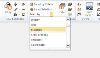
Leaving aside the graphical selection, let us first look at the simplest selection, that is, by basic criteria.
Criteria selection is the most basic type of selection – for example, when you want to select all elements of a particular cross-section or material or thickness in a modeled structure. In this case, simply select the relevant criterion, for example material, from the list. A window opens automatically in which you can enter a criterion – for example, select one or more materials from a list.
Among the many such critters available it is worth noting two: by System and by Name, as are extremely useful for a quick selection, especially if we have defined systems and subsystems and modified the default element names.
Other interesting quick selection criteria are Previous selection, which is the restoration of a previously existing selection, and Vicinity, which selects objects that are in contact with the currently selected items.
But what if we want to combine multiple criteria? Then we simply open the Select by Criteria window (for example by using ALT+S shortcut) and on each tab choose the criteria we want to use. For example, when you want to select IPE 300 and IPE360 profiles that simultaneously belong to a system called Front Structure. Just select these options from the list and press OK.
Interestingly, with a single click, you can change the default setting that selects items that meet all criteria (Intersection mode) to a setting that selects items that meet at least one of the selected criteria (Union mode). In addition, the operation can be performed on an existing selection. As you can see complex criteria are very easy to operate. As mentioned earlier, splitting the model into systems makes the work much easier. For example, when we want to select elements from a given system, we just need to do it from the Project browser level.
Using the same method, you can instantly hide or isolate a section of the model. Furthermore, you can hide/show objects (including those contained in systems) even faster simply by double-clicking on the Project browser in the list. On this picture just by few quick double clicks on the Project browser only columns and rafters are displayed.
All of these are simple operations, but they make working in Advance Design seamless because of their easy access and simple use.
Often the objects which we design require a more detailed analysis at the level of a specified fragment of the structure or element. For this purpose, often the whole object is modelled for the purpose of vertical element dimensioning, and horizontal elements such as floors are designed in a separate model, assuming their certain static scheme as faithfully as possible reflecting the global behaviour of these separated elements.
The problem begins to appear when the separated element must be loaded also with the remaining fragment of the structure, which we wanted to get rid of in order to reduce the large model. For the simplest example – I would like to analyse a complicated foundation slab – its separation from the model will not help me much, because loads which dimension it are transferred from the whole structure by means of columns or walls. The simple conclusion from this…I can isolate the slab as long as I load it according to the building scheme.
Advance Design allows you to exchange the support reactions of one model for loads generated in another model.
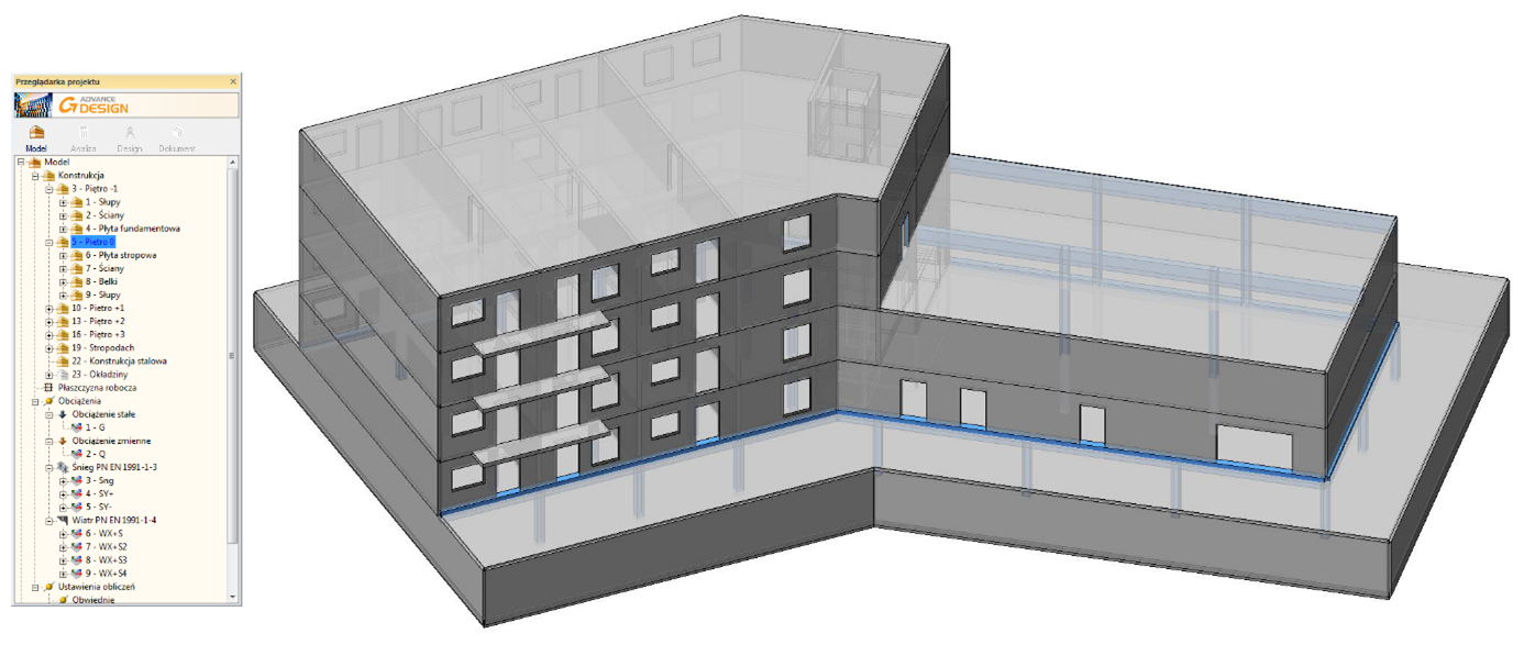
Fig. 1. Model of a simple residential and commercial building in Advance Design
At the moment I have a model of the entire building, which I can easily solve. However, I would like to divide the model e.g. into an underground and an aboveground part or into a foundation slab and the remaining part of the building. Maybe I need to analyse the foundation slab in detail and I need to reduce the size of the model to gain calculation time. Maybe I would like to divide the work into 2 workstations and leave the development of the ground slab to one of the co-workers and deal with the vertical elements of floor -1 or higher I am able to do this by creating, in a way, 2 independent models (e.g. of the said underground and aboveground part). The problem arises in the fact that the aboveground part will load the underground part, and I have just removed it from the model.
Fig. 2. Two independent FEA models
2 Foundation slab modelled on an elastic foundation, the part above the foundation slab supported by nominal rigid supports. At this point I can solve model one – i.e. the part above the foundation slab – without a problem.
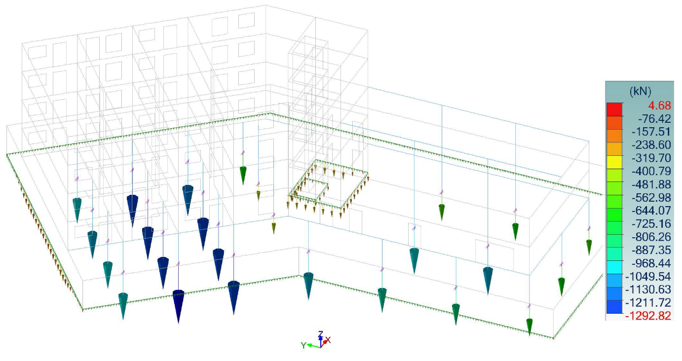
Fig. 3. Reactions (vertical) from permanent loads
Saving reactions to a file and importing them in another task
Above are examples of support reactions from permanent loads. Of course, we can transfer all reactions (displacement/rotation) from all cases.
Please note that reactions are usually presented as an inverse vector, i.e. as a response of a support – here, however, our vertical reaction is directed downwards, as it is later to be a load on a foundation slab. The reverse of reactions can be reversed by changing the program settings in the results tab by switching off the option “Include reactions on supports”. On the BIM tab, the user can export the reactions to a text file and import them into the foundation slab model in the same way. The load cases and the position of forces in space are preserved.
Fig. 4. Reactions imported into the foundation slab model
Importantly, I can import reactions at any time, meaning potential changes to the output model are not threatening. I can also modify the geometry of the foundation slab freely – the loads are not associated with it, they are in a specific space in the model and load the element underneath them. The forces are in the same load cases as in the original model so the combinations do not change. I could, however, combine the loads differently because in a smaller, detailed foundation slab design I will be able to successfully prepare more combinations.
The only thing I would like to point out is that it is necessary to separate structural elements sensibly. Their work under loads may be influenced by the elements that we have removed. That is, in addition to transferring loads, they also stiffen the component under consideration and change its working character somewhat. It is relatively correct to separate the whole storey.
This method can also lead to a kind of phasing of the structure.
Pushover analysis consists of 3 major phases, first the preprocessing phase in which the model is prepared for the analysis. Then, the processing phase during which the model is analyzed and finally the post processing phase where the results are interpreted.
1. Preprocessing phase:
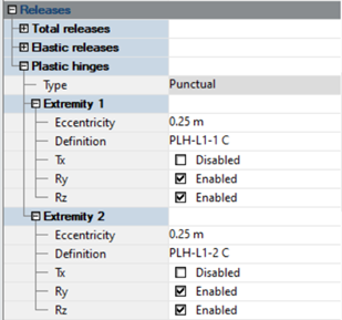
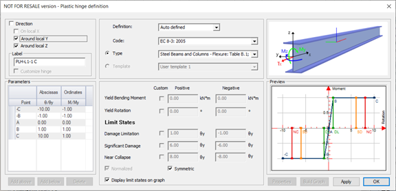
the user first needs to define the plastic hinges at locations where they are expected to occur (ends of beams), or at locations where their arise needs to be monitored (ends of columns). The plastic hinges can be defined on individual linear elements from the properties panel.
Separately for each extremity, the user is able to select the degrees of freedom for which the hinge is applicable. The ID name of a plastic hinge is generated automatically, and it consists of prefix PLH-L (plastic hinge on linear element), ID of the element, the extremity (1 or 2) and the type of the element (B – for beams, C for columns). The definition of parameters of the plastic hinge can be done by using a dialog opened by a button on the Definition property.
In a case the user decides that hinge parameters are calculated automatically, he can select the code (EC 8-3 or FEMA 356) and element type. The list of types (steel or concrete beams and columns) depending on the selected code. The content of the part with properties also depends on the selected code. Note, that some of parameters are computed during the next stage, during the pushover analysis. In case the user decides to manually define hinge parameters, then after selecting the code can unlock and edit available parameters.
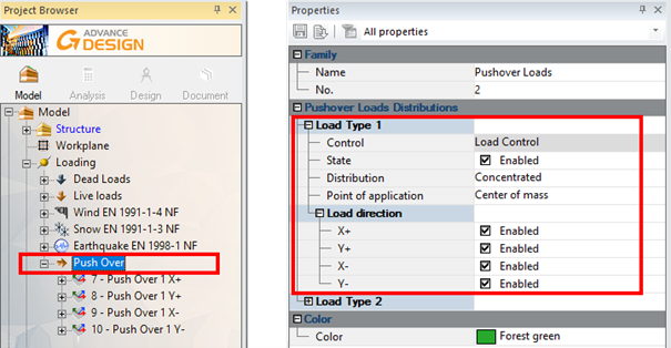
The next step is the creation of pushover load cases and generation of pushover loads. For this, a Pushover load case family type can be defined from the Create load case family. On its property list we can set the basic data for load generation such as: the distribution type, the point of application and the directions of the loads.
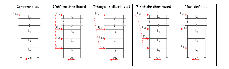
There are several load patterns available to distribute the pushover forces on the height of the structure:
Where Vb is the maximum total lateral load and Fn is the maximum lateral load applied on level n.
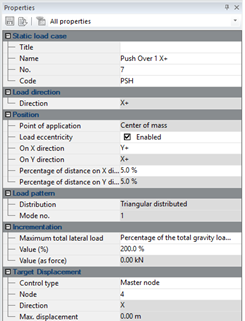
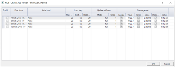
Using the right click menu on the PushOver load case family we can then automatically generate the pushover load cases and loads. On the property list of each generated pushover load case we can set details related to the maximum total lateral load and conditions for stopping the analysis.
The maximum total lateral load is the cumulated sum of the lateral loads applied on last step of the pushover analysis. This load can be defined either as the imposed value or as a percentage of the load applied on the structure prior to the pushover. For the second case we can use either the total gravity loads or the seismic base shear force on X or Y direction.
2. Processing phase:
The pushover analysis is a list of sequential actions, activated by a dedicated Pushover checkbox control in Calculation Sequence dialog
The pushover analysis is a static nonlinear analysis during which the structure will be pushed laterally until reaching the maximum specified lateral force or developing a failure mechanism.
3. Postprocessing phase:
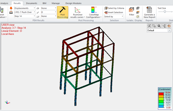
As with normal static calculations, FEM results such as displacements and internal forces are available. The results can be checked as for the non-linear calculations for each of the subsequent calculation steps.
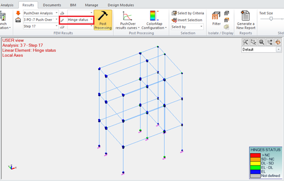
A Pushover Results entry is available on the FEM results selection that allows for selecting the Hinge status result for linear elements. When activated, it shows status of defined plastic hinges for selected step of the selected pushover case. The status is displayed by using colors.
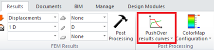
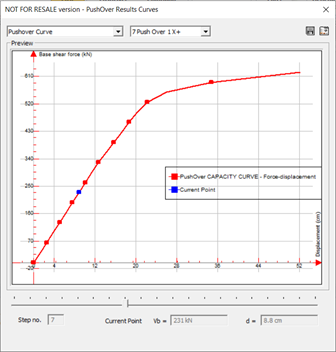
Using the Pushover results curves command, available on the Results ribbon, a pushover capacity curve can be generated. It displays a relationship diagram of the displacement of control node with respect to the total applied lateral load.
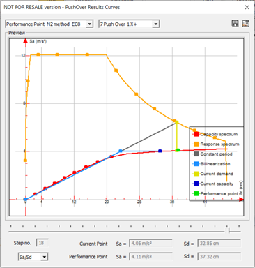
The pushover capacity curve represents the structural capacity to resist lateral loading and is a reflection on how the structure will behave when loaded laterally (seismic loads). During earthquake, the structure will be pushed laterally until a certain maximum displacement of its control node (master node). The point on the pushover capacity curve having this maximum seismic displacement is called the performance point. Physically speaking, this performance point is the balance point between the structural capacity (pushover capacity curve) and the seismic demand (seismic response spectrum). Advance Design can calculate the performance point according to the Eurocode 8 N2 method and ATC 40 Capacity Spectrum Method.
Knowing the maximum lateral displacement provided by the performance point, the user can refer to the pushover step corresponding to this maximum displacement and check the locations and limit states of plastic hinges, inter story drifts …
Graitec, as a global software editor in the Design, Structural, Fabrication, and Data Management arena organizes an international contest dedicated to structural engineers and design offices.
The award is for the best practical use of Advance Design in Steel / Timber / Concrete design projects. This contest is open to customers and students who want to showcase their experience and technical knowledge through a project executed in Advance Design software. The projects will be judged by a professional jury. The final nominees and the winning projects will be made public to a wide audience through extensive marketing including social media.
• 30.7.2021 Entries close – Deadline for project submission
• 10.9.2021 Project Confirmation – Confirmation and announcement of projects accepted
• 11.10.2021 Jury Deliberation – Selection of winners
• 19.10.2021 Announcement of Results – Announcement of winners at the Advance Design User Summit 2021
Contest criteria:
The independent contest jury will gather in October 2021 to evaluate the projects. The judging will be done under the guidance of a dedicated Graitec Group representative. The representative is in charge of the contest. The jury will evaluate the projects taking the following criteria into consideration:
Technical level of the design, detailing and/or calculations.
Originality and prestige of the project.
Attractiveness, detail and presentation of the project.
Optimal use of software’s functionality.
The “story” behind the project – difficulties overcome, innovative approaches, benefits gained, etc.
Jury:
An independent and international jury composed of academics and professionals in the field will judge the submitted entries. Meet the members of our jury:
Francis Guillemard – Jury Chairman / GRAITEC President of the Group and Chairman of the board / France
Rawad Assaf / ISSAE – CNAM Liban/ Lebanon
Olivier Chappat / Bouygues Bâtiment Ile-de-France / France
Piotr Nazarko / Rzeszow University of Technology / Poland
Rodrigue Coyere / EIFFAGE CONSTRUCTION Structural design office / France
Daniel Bitca / Technical University of Civil Engineering Bucharest / Romania
Jiri Bendl, GRAITEC, Vice President SIMULATE comments: “Through the Advance Design Award organizations we want to reward our customers for being members of the ever-growing SIMULATE community and we want to encourage students to use the best possible tools for structural analysis. It is a great pleasure for me to be part of this project!”
About GRAITEC
Founded in 1986, GRAITEC is an international group (13 countries worldwide – 48 offices) helping construction and manufacturing professionals to successfully achieve their digital transformation by providing BIM and Industry 4.0 software and consultancy. GRAITEC is a developer of high-performance BIM applications as well as an Autodesk Platinum Partner in Europe and Gold Autodesk Partner in North America and Russia. With more than 550 employees including 200 BIM consultants, GRAITEC is an innovation-focused company whose products are used by more than 100,000 construction professionals worldwide.
According to EN1993-1-3, formula (10.1b), the shear stiffness of trapezoidal sheeting connected to a purlin may be calculated as :
With:
t : thickness of sheeting (in mm)
broof: width of the roof (in mm) (roof dimension parallel to the direction of the panel ribs)
s: spacing between purlins
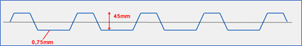
hw: profile depth of sheeting
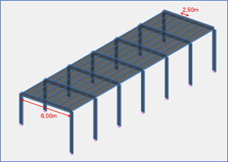
Assume a purlin connected to the following trapezoidal sheeting, at each rib:
Roof width : 6,00m
Distance between purlins : 2,50m
This result sin a shear stiffness of 8361 kN.
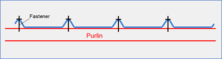
Formula (10.1b) assumes the purlin is connected at each rib to the trapezoidal sheeting :
Purlin connected at each rib
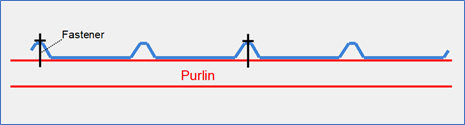
In case the purlin is not connected at each rib but at every other rib, only a small portion (20%) of this S stiffness can be considered :
Purlin connected every other rib
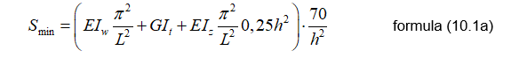
If this value exceeds a certain value (Smin), the purlin may be regarded as laterrally restrained in the plane of the sheeting.
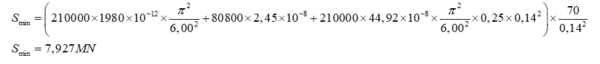
Assume an IPE140 purlin:
Iw = 1980 cm6 (warping constant of the purlin)
It = 2,45 cm4 (torsion constant of the purlin)
Iz = 44,92 cm4 (minor axis inertia of the purlin)
h = 140 mm (height of the purlin)
L = 6,00m (span of the purlin)
In our case, S > Smin. The condition is met and the purlin may be regarded as laterally restrained.
In Advanced Design, such a purlin may have its ‘Continuous restraint along flange’ property enabled on the upper flange :
For more complex cases, when the member is prone to torsional effects (Channel or Z section for example), a more sophisticated calculation may be required (2nd order calculation with warping).
In this case, the shear stiffness (S) may be taken into account as the ‘Shear field’ parameter from the ‘Advanced stability’ dialog :
ArchiWIZARD allows a link with all the BIM solutions on the market thanks to a direct import in IFC format, SketchUp format and in REVIT format. ArchiWIZARD is responsible for the automatic creation of the energy model (rooms, walls, bays, thermal bridges, environmental elements) from the 3D digital architectural model. This common energy model is used for all ArchiWIZARD’s simulation engines.
Figure 1 – Environment ArchiWIZARD
A. REVIT model import ArchiWIZARD has a standalone version and a direct ArchiWIZARD plug-in in REVIT. The 3D model is exported by the geometric analysis in the ArchiWIZARD standalone version, and with the REVIT energy model in the ArchiWIZARD plugin of REVIT (process called BIM import).
Figure 2 – Two types of import
• Geometric analysis Import: This is a simple geometry analysis of the 3D model. ArchiWIZARD will detect these closed volumes and it creates the project walls accordingly. This geometric analysis will be used to generate an energy model adapted to the module used in ArchiWIZARD (Real-time module, STD module, Regulatory modules, etc.).
Figure 3 – Import by geometric analysis
• REVIT BIM import: This feature can only be used in the ArchiWIZARD version integrated with the plug-in REVIT software and allows to generate an energy model based on parameters (location, wall compositions, materials and their thermal properties, name and room dimensions, among others ) from REVIT energy model and, of course, to get access to all ArchiWIZARD features.
Figure 4 – REVIT energy model preview in gbXML
B. Real time data synchronization ArchiWIZARD and REVIT models are linked and some properties like thermal properties are synchronized in real time without having to synchronize.
Figure 5 – Parameter synchronization in real time
Display results in REVIT
Some ArchiWIZARD results may be displayed in the current Revit view such as light range, light comfort or thermal loads EN12831.
Figure 6 – ArchiWIZARD solar imagery generated in REVIT view
D. Access to all ArchiWIZARD features and interface
All ArchiWIZARD functionalities are accessible and operational in the Revit environment via the control ribbon.
Figure 7 – ArchiWIZARD control ribbon in REVIT view
Working with the ArchiWIZARD plugin gives access to both software simultaneously. The constant exchange of information in this BIM environment allows to optimally enrich REVIT’s 3D model as well as the ArchiWIZARD’s thermal model.
One of the benefits of the Railing macros, available in PowerPack for Advance Steel, is that the library of profiles used to create the railing can be extended.
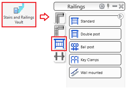
In other words, the user can add any section to the Railing macros from the Stairs and Railing Vault.
This feature is available starting with version 2021.1 of PowerPack for Autodesk Advance Steel.
Stairs and Railings Vault
All the Graitec railing macros can be configured to use records from the Autodesk Advance Steel AstorRules database – JointsGUIAllowedSections table. This behavior is like some Advance Steel standard joints.
This flexibility of the macros offers the users to go beyond existing restrictions and extend the list of available sections in the profile selection controls, for each type of main railing element such as:
post
top rail
middle rail
kick rail
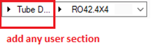
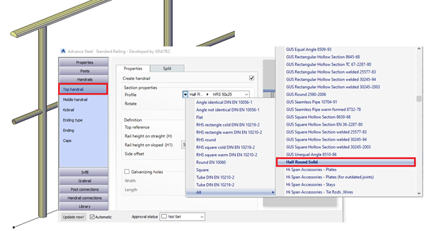
Profile selection control inside the dialog
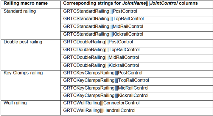
To make this work, the following strings (names) for the JointName and JointControl columns in the table, for each railing macro and each main element type inside the macros, must be used:
How it works?
Open the Table Editor from MANAGEMENT TOOLS – AstorRules database – JointsGUIAllowedSections table.
Create a new table entry for the desired user section.
Add a new entry inside JointsGUIAllowedSections table:
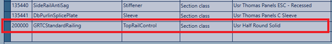
Example: add half round solid sections to be used for the top handrail inside the Standard railing macro
New entry in JointsGUIAllowedSections table
Update the database and reload it in Advance Steel using the Reopen database option. Next time the Standard Railing macro is opened, the new type of profile section can be used inside the railing: