PowerPack for Advance Steel Stair Macros – Understanding the Philosophy


The Stair macros available with PowerPack for Advance Steel are powerful tools for anyone who wants to create stairs, but they are not magic.

To get the best from these macros it’s important to understand the philosophy of how it’s working. This philosophy is based on 4 aspects that you must have in mind before using the macro.

Let’s start with the first one.

A. The 2D setting out points defined

To ensure the macro works as expected, you need to have the 2D setting out points defined.

This is an important step to be done before starting the modeling.

The PowerPack Premium Stair tools use different setting out points. You need the bottom point of the first tread & top point of the last tread, exactly how is showed in the image below.

B. Don’t forget about the overlap

If your stair has a constant overlap, then move your last point horizontally to include the overlap.

In the example below the overlap is 50mm, therefore the blue point was moved with 50mm.

C. Know the length of the landing extension

For the staircases with 2 or 3 flights you need to know the length of the landing extension before using the macro.

In the example below, you can see 2 landing extensions for a stair with 2 flights: one of 230 mm in blue and the second of 460 mm in red.

D. Turning points for multiflight stairs

For the multiflight stairs created with the PowerPack macros, you need to define the turning points at the ground level, as you can see in examples below.

Going through these 4 steps before starting to use the Stair macro, will ensure that the macro is working as you expected and you will get the full benefits of its features.

How to activate “Advance stability” analysis on steel elements in Advance Design


In order to perform second order analysis on steel elements in Advance Design, Steelwork Design “To calculate” option must be activated from the element’s property list.

Figure 1 – Steelwork Design Activation

This feature is available either for each individual steel profile or for a multiple selection, by checking 2nd order with warping and imperfections checkbox, setting the Number of iterations and Stability 2nd order parameters.

Figure 2 – Advance Stability Activation

The “Advanced stability (2nd order)” parameters can be found in the Steelwork Design section of the property sheet for steel members. 

Figure 3 – Advance Stability Options

(1)    Checking the “2nd order with warping and imperfections” box will perform the analysis of the selected members during the steel calculation sequence. 
(2)    The 2nd order analysis being an iterative process , the user can set the maximum number of iterations. 


The 2nd order analysis uses the user-defined imperfections in order to determine the final 2nd efforts. The imperfections are applied step by step, incrementally, until the final imperfection defined by the user is achieved. At every iteration, the 2nd order efforts are recalculated starting with the previously calculated efforts. Calculations are made until convergeance – defined as the difference between 2 succesive iterations (automatically managed internally by the solver) – is achieved,  or until the maximum number of iterations is achieved. 


(3)    The “Stability – 2nd order parameters” will give access to a dialog where the user can define the various parameters to be considered during the analysis of the selected members. 
The definition dialog will show 4 tabs: 
•    Nodal springs
•    Bedding
•    Imperfections EC3
•    Loads offset

Figure 4 – Advance Stability Assumptions

Vistit Advance Design LinkedIn page HERE

Visit Advance Design Virtual Stand HERE

Get Advance Design FREE TRIAL HERE

How to define nodal springs in “advance stability (second order analysis) solver


Although the “Advanced stability” from Advance Design feature considers the individual member, the intersections with the other elements are of course taken into account. In fact, the intersections are turned into nodal springs

Figure 1 – Auto Detect Spans Option

The selected member has intersections with other elements at x = 0.00m and x = 4.00m.

The “Auto-detect spans” button enables the users to see the intersections and alter the behavior of the corresponding springs.

The users can also add or delete nodal springs (only user-added nodal springs can be deleted) from the grid using the “Add” and “Delete” buttons. Moreover, they can reset the grid with the help of the “Reset” button.

Note: Even if the user does not open the Advance stability definition parameters, Advance Design will automatically take into consideration the intersections with the other elements during the analysis.

Note: If geometrical parameters are modified after the “Advance Stability” option is checked for steel members, “Reset” and “Auto-Detect Spans” options must be selected in order to reinitialize the position of the nodal springs. Any modifications made in the Advance stability window will be reset to default. Otherwise, the calculation will not be successful.

For each nodal spring, the user can set the status for each of the seven DOF.

    TxTy and Tz stand for the displacement along the x, y and z axes respectively 

    RxRy and Rz stand for the rotation about the x, y and z axes respectively

    Rw is the warping

Figure 2 – The seven Degrees of Freedom

Available statuses are:

  • Free: enables the release for the considered degree-of-freedom ;
  • Fixed: disables the release for the considered degree-of-freedom (this translates into a very high stiffness);
  • Auto: lets Advance Design automatically determine whether the degree-of-freedom is free or treated as an elastic release (the stiffness of which is automatically computed by Advance Design for each combination);
  • Elastic: defines an elastic release for the considered degree-of-freedom (stiffness imposed by user).

When set on “Auto“, Advance Design is able to compute the appropriate stiffness of the release as Force/Displacement, resulting in a stiffness value for each combination.

 Figure 3 – Stiffness definition

Warning: the “Auto” status means that the “Advanced stability” feature will attempt to re-create the boundary conditions based on the Forces and Displacements diagrams from the global model.

This can be challenging in some cases as the automatic determination has its own limitations.

For example, zero forces on a given node can either mean:

  • The degree-of-freedom (DOF) is free;
  • The DOF is fixed but no force was acting in the given direction.

Therefore, we would advise the users to manually set the free DOF”s on “Free” whenever possible as the “Advanced stability” feature is not able to import the boundary conditions defined on the member in the global model. The “Advanced stability” feature can only deduce the boundary conditions from the Forces and Displacements diagrams it imports from the global model.

We would also advise the users to make sure the member does not feature a free “Rx” DOF on both ends as this could lead to a numerical instability if no other intermediate nodal spring exists.

Setting the “Rx” DOF on “Fixed” can be a solution when the “Auto” detection method fail.

Figure 4 – Degrees of Freedom Status

The “Position” property enables the user to define an eccentric spring.

Eccentricity is meant in the z direction (Upper fiber, Neutral, Bottom fiber or User value).

Figure 5 – Nodal Springs Position Eccentricity

Stiffness auto correction 
There are cases when, by activating the “Auto-detect spans” option, the automatically calculated stiffness does not meet the minimum criteria in order to successfully perform the 2nd order analysis (for example, when displacements are automatically imposed at an element”s ends for which the automatically calculated stiffness is insufficient). By activating the “Stiffness auto correction” option, the program automatically imposes a minimum stiffness in order to successfully perform the analysis, but only when the values are very small.

Figure 6 – Stiffness Auto Correction Activation

Generally, the warping DOF (degree-of-freedom) is free and fixing it requires special rules for detailing, like the end plates, beam extensions, flat stiffeners.

Vistit Advance Design LinkedIn page HERE

Visit Advance Design Virtual Stand HERE

Get Advance Design FREE TRIAL HERE

How to analyze irregular reinforced concrete cross-sections?


The reinforced concrete linear elements are usually characterized by square, rectangular or circular cross-sections. Advance Design computes the reinforcement for such elements with the Reinforced Concrete (RC) Design expert. For irregular, user defined cross sections, the RC design falls outside the standard procedure. Therefore, the real reinforcement may be determined following an iterative process, as described in the next steps:

1. Add a new user defined cross-section – follow the steps from Figure 1

Figure 1 – Steps to define a new user section

2. Define the cross-section geometry (shape and reinforcement position) and material in the Cross Sections module: draw the shape by point coordinates, define the reinforcement (automatic or manually) and concrete cover, define the material and calculation settings.

Note: It is recommended to define the initial reinforcement from the minimum reinforcement area.

Figure 2 – Define the cross-section shape and place the reinforcement

3. Set parameters and calculate the cross-section properties

Figure 3 – Calculation settings

4. Export the cross-section to the Advance Design library

Figure 4 – Close and export the cross-section to Advance Design library

5. The user defined section is attributed to the desired linear elements (columns). Run FEM and RC Design analysis.

6. On the selected element, check the RC design – element reinforcement results. The real reinforcement (imposed) can be compared to the theoretical reinforcement (computed). The verification can be observed on the interaction curves also. The section solicitation point should fall inside and close to the capacity curve (My/Mz, Fx/My, Fx/Mz), for a safe and economic design. If the imposed reinforcement does not satisfy these conditions, the initial reinforcement is increased: restart from Step 2.

Figure 5 – Check the proposed reinforcement

Graphical model validation by displaying it in colors in Advance Design


In this short article, we will look at one of the model validation methods available in Advance Design – displaying modelled elements in color according to selected criteria. Although this functionality is more general and can be used simply to improve the way a model is presented in a view or for documentation, today we will focus on its advantages for model verification.

Let us start with the topic of verification of local system of axes of surface elements. Checking and eventual change of local systems is an important step in the verification of the model, because by proper arrangement of local systems we have control over the uniformity of the FEM results and the reinforcement directions. Each modelled planar element has its own local system of axes, which is set automatically. Knowing the basic rules of automatic local axis system setting (as for example that the x-axis of the local system is usually defined along the first edge of the drawn contour) we can often control it ourselves. However, this is not always convenient or possible, especially when the model has been imported. Checking the local layout of axes for one or more elements is not a problem – we can simply select a surface element and we see its local axis symbol by default. The colors of the axes correspond to the colors of axes of the global coordinate system, i.e., the red axis is local x, the green one is local y and the blue one is local z.

However, it is much more interesting how we can quickly check the local axis settings for a larger number of elements / for the whole model.  To do this in Advance Design, we can use a very versatile tool to display objects in color according to selected criteria, available in the Display Settings window. In the ‘Color’ command group, there is a list for selecting coloring criteria, as well as additional options including displaying a legend and displaying the element’s local system axis during element selection.

For our purposes, of the many criteria available here, three will be useful to us: Local x orientation, Local y orientation and Local x orientation. All these modes are used to indicate in which direction the axes of the local system are oriented relative to the global system.

Take a look at the image below showing an example of the effect of using the ‘Local x orientation’ option.

The surface elements are colored and thanks to the legend we can immediately see how the local x-axis is oriented. For example, dark blue means that the local x-axis is pointing in the Y- direction of axis of the global system, light blue means that it is pointing in the Z- direction (down), while red means that it is pointing in the Z+ direction (up). We can easily confirm this just by selecting elements, as then we can see symbols of local systems.

If we now want to unify the orientation of the local axes, all we need to do is select the relevant elements, which is very easy thanks to the colors, and then choose one of the dedicated commands: Local Axis or Local Axis on direction.

On a similar basis, we can verify the orientation of the other axes of the local system of planar elements, but in the same way we can verify the local systems of linear elements. Of course, for this purpose, it is best if we filter out only the linear elements for presentation. But the same types of coloring styles as for surface elements can be used for this purpose.

The layout of local axes is not all that we can verify with coloring. The same tool can be used to verify the correctness of the modeling according to other criteria – for example thicknesses.

On the same principle, we will also check the cross-section of linear elements or the material that has been assigned to different elements of the model. But that’s not all. In a similar way, we can color elements according to their type, system assignment, or super element affiliation. And, other objects, such as loads by category or steel connections by type.  I recommend that all Advance Design users become familiar with all the available coloring criteria because using them increases the control over the model.

Learn more about Advance Design!

How to simulate membrane behavior in Advance Design using DOF constraints?


In order to simulate the membrane effect in a structure in Advance Design, “DOF (Degree of freedom) constraint” object can be used with the Tx and Ty translations restrained.  DOF constraint object is also named as Master-Slave connection. The command can be found in “Objects” ribbon tab:

Figure 1 – DOF constraint localization

The following properties regarding restraints definition are defined for the “DOF constraint” (Master-Slave connection):

Figure 2 – DOF constraint properties

For example, the response of the DOF constraint is compared with the response of a membrane in a simple 3D structure subjected to lateral loads. In this model, the elements’ self-weight is not considered.

Figure 3 – DOF constraint model view
Figure 4 – Membrane model view

Since the master-slave connection imposes to all component nodes the same DOF restraints (translations/rotations), the master node can be placed anywhere on the perimeter. In order to simulate the same response, the nodes must be placed on the same position as the mesh nodes of the membrane:

Figure 5 – DOF constraint mesh view
Figure 6 – Membrane mesh view

The similar response of the two objects (master slave connection with Tx and Ty translations restrained and membrane) can be verified by comparing the results of the FEM analysis:

Figure 7 – Displacements comparison between the two models
Figure 8 – Axial force comparison between the two models
Figure 9 – Bending moments on columns comparison between the two models
Figure 10 – Bending moments on beams comparison between the two models

Learn more about Advance Design!

Join BIM WORKFLOW WEEK!


BIM WORKFLOW WEEK is an online event organized by GRAITEC for structural engineers and detailers. Nowadays, you can streamline your BIM workflows using Graitec and Autodesk technologies together. Bridge the gap between all stakeholders and discover how you can develop and improve your construction projects in a digital thread!

Each day we will run a webinar to show how easy it is to streamline your daily work! We show how to apply a complete BIM workflow from design to detailing on all your projects during the webinars! Don’t wait and register today!

BIM WORKFLOW WEEK AGENDA:

Monday – 15/03/2021 – CREATE YOUR BIM MODELS WITH REVIT AND SIMULATE THEM WITH ADVANCE DESIGN

Are you a structural engineering company doing construction projects with Revit® from Autodesk in a BIM environment? In this webinar, we will propose you a way to streamline your projects, starting to CREATE BIM data in Revit, exporting it to Advance Design to SIMULATE your building and synchronize back in Revit all changes. Discover how easy it is to link Autodesk Revit and Graitec Advance design to simulate and optimize your steel an concrete projects.

Tuesday – 16/03/2021 – ENRICH YOUR 3D BIM REVIT MODEL WITH ANALYTICAL DATA AND RESULTS USING ADVANCE DESIGN

In this webinar, we will go deeper in the integration between Autodesk Revit and Advance Design: exchanging and synchronizing geometrical data is a good point but is not enough to enable a real BIM structural workflow. During this session, you will discover how to enrich your Revit model with finite element results and theoretical reinforcement values using Advance Design with an effective synchronisation mechanism controlled by the user!

Wednesday – 17/03/2021 – APPLY AN EFFECTIVE BIM WORKFLOW FOR ALL YOUR REBAR PROJECTS IN REVIT!

In this BIM era, it’s time for you to manage your rebar projects with 3D models using Autodesk Revit®! Join us to this webinar and discover how you can use the Autodesk platform and Advance Design together to produce 3D Design-driven rebar cages for Beams-Columns-Footings-Slabs-Walls & Shear Walls, automate the drawing views creation with all tags and annotations, produce final drawings and manage in real time all your rebar projects!

Thursday – 18/03/2021 – STEEL CONNECTIONS DESIGN REINVENTED FOR ADVANCE STEEL USERS!

If you’re a structural engineer or a steel detailer using Advance Steel and want to save time, cost and reduce your carbon footprint, Graitec now offers a solution to complement and optimise your current workflow. To facilitate analysing these complex 3D steel connections, Advance Steel joints can now be exported to Graitec Advance Design Connection!

Friday – 19/03/2021 – APPLY A COMPLETE BIM WORKFLOWS FROM DESIGN TO DETAILING ON ALL YOUR STEEL PROJECTS!

In this webinar, we will go through a complete BIM workflow from design to detailing using Autodesk Advance Steel and Graitec Advance Design together. You will discover how easy it is to design and optimise a steel structure with Graitec Advance Design, including steel joints. Then, we will end by exporting the model to Advance steel to create drawings, BOM lists and CNC files fir the fabrication.

How to optimize steel elements in accordance with the deflection criterion?


The shape optimization calculation for steel elements can be performed in Advance Design  considering the condition of maximum deflection. Then, new cross-sections are searched if the deflection ratio is greater than the set limit (default 100%).


Thanks to this option from Advance Design, it is possible to optimize steel elements while using more criteria at the same time, like searching and selecting for profiles that must meet the conditions for maximum load capacity (strength/stability) and maximum deflection, independently or at the same time. This is especially useful for design of steel structural elements that exceed the maximum deflection while meeting the load capacity condition.

The optimization assumptions can be found in the Optimisation tab from Steel Design Calculation Assumptions dialog. Under the “Find new sections” paragraph, a new option is available to activate the deflection criterion and to set the maximum allowable deflection ratio considered for the cross section optimization. These assumptions apply to all steel members from the model which have Steelwork DeDefault optimization assumptionssign option from the element’s properties activated. The limits imposed in this tab apply to all cross sections as a group and cannot be applied differentially for singular element.

By default, the deflection ratio optimization is unchecked:

Figure 1 – Default optimization assumptions

By checking the “if the max/all deflection ratio is greater than:” option, the user can impose the maximum ratio.

Figure 2 – Activation of the deflection optimization criterion

Once the steel calculation is completed, the strength/stability and deflection work ratios of steel elements are compared with the specific criterion, and other cross sections that meet the imposed conditions are suggested.
The results of steel elements optimization are displayed in the Suggested shapes dialog, displaying the current strength/stability and deflection ratios. If the ratios are greater than the imposed limits (100% by default), the current ratio is displayed in red. For such cases, if the deflection criterion is activated, the next cross section from the catalog that will meet the required criterion will be suggested, displaying also the ratio for that section.

Figure 3 – Suggested shapes according to selected criterion

By opening the Accepted solutions flyout, we can select the suggested shape or other section from the same catalog.

Figure 4 – Selection of accepted solutions

After accepting the suggested (or imposed) sections, from the Accept all option, a new steel calculation is required, in order to recalculate the new sections and have correct results in the shape-sheet of the elements and reports.
This optimization sequence is directly dependent with the sorting mode selected in the Sort profiles tab from steel Calculation assumptions. By default, the “Envelope criterion” option is selected, which means that the suggested profiles will meet both deflection criterion and strength/stability criterion.

Figure 5 – Default sort mode for section optimization

If the Envelope criterion is selected, the new profiles are suggested from both cases, if the deflection or strength/stability criterion are exceeded:

Figure 6 – Suggested shapes according to envelope criterion

If the Deflection criterion is selected, then the new profiles are suggested only if the deflection ratio is exceeded:

Figure 7 – Suggested shapes according to deflection criterion

If the Strength/stability criterion is selected, then the new profiles are suggested only if the deflection ratio is exceeded:

Figure 8 – Suggested shapes according to strength/stability criterion

In order for the deflection criterion based optimization to be computed, both Steelwork Design and Deflections options from element’s property list must be checked. The optimization based on deflection will be made according to the parameters introduced in the property list:

Figure 9 – Element property check


If the deflection verification is unchecked for an element, then “N/A” (Not available) message will be displayed for the Deflection work ratio in the Suggested shapes dialog.

This new feature makes result checking easier, thanks to the possibility of presenting a ratio for deflection during shape optimization. It also gives you the possibility to select optimal steel profiles considering the deflection. Various options from the Assumptions dialog help you get specific results for the steel elements used in design and enhance the workflow.

Learn more about Advance Design!

Advance Steel SDNF export – how and where to create new entries?


Recently this question came up from a colleague on how and where you find the Database entries behind the SDNF Export from Advance Steel.   So, this is what is behind todays idea for the blog.  

Within Advance Steel there are many different types of Export/import options, the core one of these is the SMLX options for transfer from Advance steel to Revit to Advance Steel, but sometimes over more traditional export formats are needed, in this case the SDNF format (Steel detailing neutral format) was being used to link to a Steel and piping software, the user was using Advance steel to complete their steel process but wishes to update within their piping platform. The simple answer is that the SDNF export uses the Databases called the GTC mapping, but which one, as there are two locations and then which tables, as there are several within the database. So, with this goal in mind, we looked into the actual database and more importantly which table and how the entries in the table are completed.   The conclusions of this and approach is explained in the attached document link, but the summary is that for the export process the GTC mapping database, that is located under the Advance folder of Autodesk within your program files, is where you need to look and it is using the table called the ‘Profile Export conversions’, under the Advance Steel type. Also, the entries for the table can be created using the ‘Autodesk one to one mapping’ or can use the ‘expression format’ that is common within the database entries.

Advance Steel SDNF Export Mapping

Using Advance Steel 2021 version and the for the Export to SDNF option via the ribbon, we look at how to make a section group into the Export systems.

Which Database

For the SDNF mapping the database is the GTC mapping.MDB database, this is found under the Advance\data folder of Autodesk within your program files.

C:\ProgramData\Autodesk\Advance\Data

Note: to see this you may have to enable hidden files and folders under the windows explorer options.

The data base is an Microsoft access database, the best way to edit this is with ‘Access’.

Which Table/s

So the heading says which tables, for good reason, the system actually uses the Profile Export conversion table:

Although if you are creating entries via the mapping dialog that appears in the software, if it finds a beam type not mapped previously, in that case it creates two entries, with the other being in the GTC profile conversion.  If you do create entries manually, you can go in and remove these, as they are not used.

How to find an entry in the table.

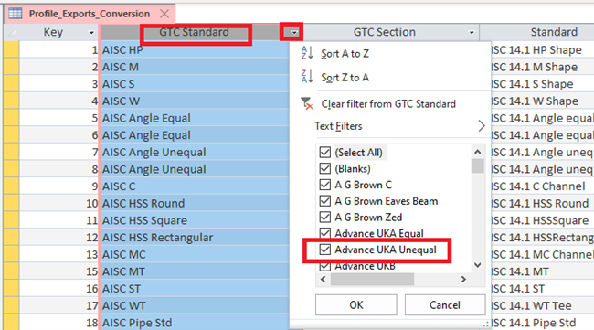
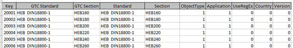
For the Access field , you can filter this down by checking the box under the column filter to show only those elements:

In this case just uncheck select all, then scroll the list and check for example HEB

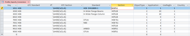
You will see several listings for HEB, some with different GTC standard and export applications listed.

But actuall none of these may be any good to export exactly what you need.  For example the line 1011 would look good for this export to SDNF,  but trying this it is not doing what you would expect.

The issue is coming from the  GTC standard, this does not have the correct reference that is aligned to the entry in the profile master table. That is the tynename text used in the profile master table, under the astorprofiles database.

The HEB reference is using the other table, and obsolete one.

The solution

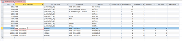
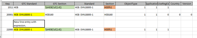
The easiest way round this is to create a new table reference, to reflect the correct string and references,  so you can either manually do this, or maybe just take a few sections and map them, and look for the entries in the DB table,  they should start with prefix of 20000.

By mapping these manually, the GTC standard is created , so you can use this to form the string required.

If you have Excel this is an ideal platform in which to do this and create them and copy and paste back into Excel.

So, this is the simple way to create a line entry, then copy it out, then use the functions of Excel and expand the entries to cover all the sections from the profile table.  This can take some time to create, but more importantly they add lots of entries to the main DB.

But there is another way to reduce this input.

Single line entry using Expressions

Within the GTC database, the user will notice there are entries, which appear to use a code abbreviation, a formula so to speak.

 These expressions come from a format called regular expressions and there is some good information on this via this website link:  ‘learn RegEx Experssion  this website very useful, very good step by step tutorial.  Take note there are many websites that explain this concept so feel free to google it and suggest others.’

This example the HEB beam mapping.

So from the previous entry in the profile export conversion table we can see the expression elements used in the line, so whilst in Access you can copy the line and paste it into Excel changing the key value to a more suitable entry, then comparing this to the manual lines, we can create a combined entry and paste it back into the Access table.

So with this line pasted back into the Access database, then close any open session of AS, close the access Database, Open the Profile export conversation table, then paste in the new entry, copied from excel.

Using this/ testing.

Create a simple model of the sections in question, then with new session of Advance steel open,  run the process for using these new entries. Select the SDNF button and process the HEB thorough the new table entries. If this is understood correctly and we run the export and the Advance steel mapping is present the process should complete within out the need for one-by-one map process.

The output

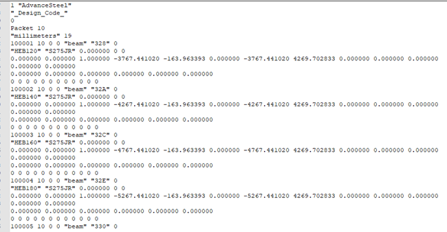
Checking the SDNF file format and naming etc, your notepad of notepad ++, you can view the file and see the names created in the listing.

All this from one line in a table, this is the process used, beyond the manual mapping of sections, it is also used for the Revit transfer of objects via the SMLX format, again using these expressions to map multiple entries.  Please see the Autodesk University class that I had the privilege to present, over the Revit AS workflow, you see the same in this class for Revit and AS.

https://www.autodesk.com/autodesk-university/class/Steel-Fabrication-Transfer-Revit-Advance-Steel-Under-Hood-2019